Import Required Routines
# For Jupyter notebook only, specifies plots are not inline
%matplotlib qt
# Imports both matplotlib and numpy routines
%pylab
from mapping.plot_map import *        # Imports plot_map and other helper routines for dealing with plots
from mapping.transform_map import *   # Imports sub_map, rot_map, drot_map
from mapping.fits2map import *        # Imports fits2map and downloading functions for creating maps
Create maps from fits files using fits2map
The first three files are downloaded from internet URLs, although once they are downloaded and found on the local disk the download is skipped. The three EOVSA maps are appended to a Python list. The two aia files are downloaded from the LMSAL Sun Today page using the get_aia_daily() convenience function. The replace=True means if a local file exists, replace it.
filename = 'http://www.ovsa.njit.edu/fits/synoptic/2020/06/05/eovsa_20200605.spw02-05.tb.disk.fits'
eomaps = []
eomaps.append(fits2map(filename))
filename = 'http://www.ovsa.njit.edu/fits/synoptic/2020/06/05/eovsa_20200605.spw06-10.tb.disk.fits'
eomaps.append(fits2map(filename))
filename = 'http://www.ovsa.njit.edu/fits/synoptic/2020/06/05/eovsa_20200605.spw11-20.tb.disk.fits'
eomaps.append(fits2map(filename))
aia211 = get_aia_daily('2020-06-05', wave=211, replace=True)  # Convenience function
aia304 = get_aia_daily('2020-06-05', wave=304)
Create a new map of column emission measure
Calculates the column emission measure for all three maps and then averages them.
from copy import deepcopy
newmap = deepcopy(eomaps[0])  # Duplicate first EOVSA map as template
newmap['id'] = eomaps[0]['id'][:12]+'-'+eomaps[2]['id'][6:]   # Update ID to show frequency range
newmap['data'] *= 0  # Zero out the data
# Calculate the column emission measure for each map and add to newmap's data, then average
for m in eomaps:
    frq = float(m['id'][5:11])*1e9
    newmap['data'] += (m['data']-10000)*frq**2*1e3/(9.786e-3*log10(4.7e10*1e6/frq))
newmap['data'] /= 3
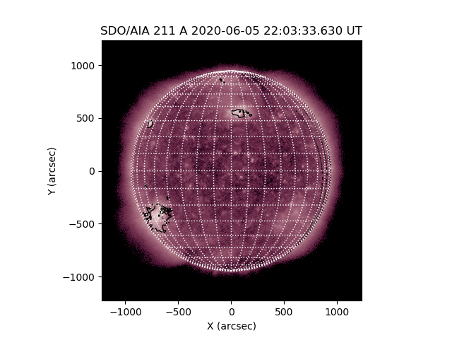
Plot the AIA 211A map and overplot with EOVSA emission measure contours
First loads all of the AIA colormaps. Then plots the aia211 map and solar grid, with log color scale. Then overplots three levels of emission measure contours, differentially rotating so the times match. This plots the entire solar disk, which can then be zoomed or panned with the Python plot tools.
aia_lct('all')
plot_map(aia211,cmap='aia211',grid=10,log=True,dmin=10)
plot_map(newmap,over=True,levels=[1e28, 5e28, 1e29],drotate=True,linewidths=1)
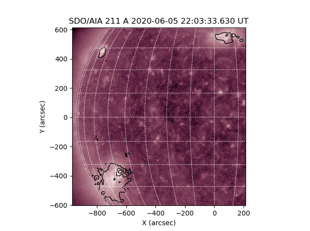
The commands below repeat the plot, but this time specifying a center, field of view (in arcmin), and that the plot should be put in a new window (window 2)
plot_map(aia211,cmap='aia211',grid=10,log=True,dmin=10, center=[-370,0],fov=[20,20],window=2)
plot_map(newmap,over=True,levels=[1e28, 5e28, 1e29],drotate=True,linewidths=1)
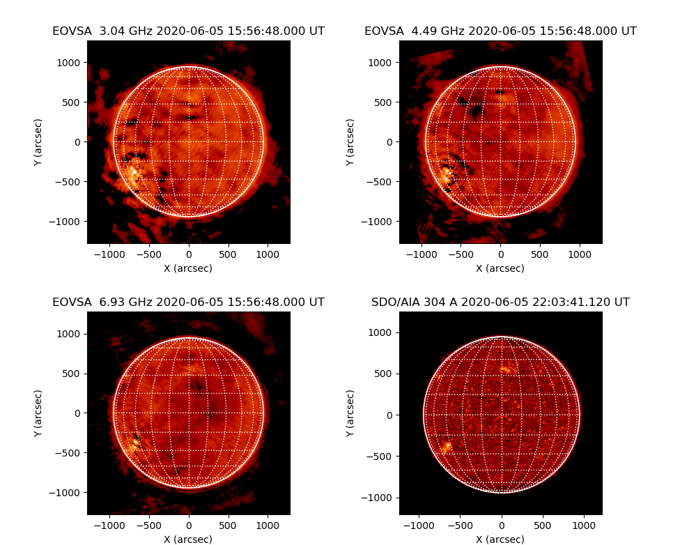
Multi-panel plots
The first command makes the aia304 colortable the default, then the first plot opens a new window (3) with four panels (2 x 2) and plots the first EOVSA map. Subsequent maps are plotted advancing panels each time. The AIA data are smoothed with a 3 pixel gaussian. The tight_layout() command improves the layout and eliminates overlap of text.
aia_lct(304,load=True)
plot_map(eomaps[0], multi=[2,2], window=3, grid=15, limb=True, dmin=1e3, log=True)
plot_map(eomaps[1], grid=15, limb=True, dmin=1e3, log=True)
plot_map(eomaps[2], grid=15, limb=True, dmin=1e3, log=True)
plot_map(aia304, log=True, dmin=1, smooth=3, grid=15, limb=True)
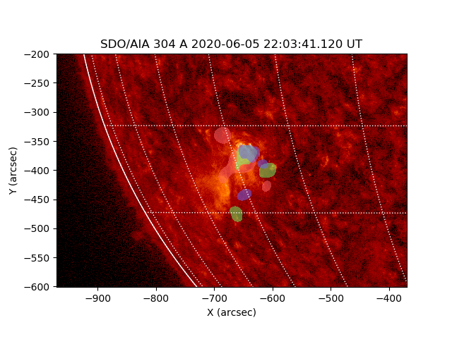
Sub-maps and filled contours
The first command creates a new map that is a cut-out from the AIA 304 map, plots it, and then overlays red, green, and blue 50% contours from EOVSA maps, suitably differentially rotated.
saia = sub_map(aia304, xrange=[-970,-370], yrange=[-600,-200])
plot_map(saia, window=4, log=True, grid=10, limb=True, dmin=1)
plot_map(eomaps[0], over=True, color='#ff666680', fill=True, levels=[50,100], percent=True, drotate=True)
plot_map(eomaps[1], over=True, color='#66ff6680', fill=True, levels=[50,100], percent=True, drotate=True)
plot_map(eomaps[2], over=True, color='#6666ff80', fill=True, levels=[50,100], percent=True, drotate=True)
Below is an example of direct differential rotation of the above submap to a time some two days later. The track_center parameter shifts the map center to follow the rotation.
daia = drot_map(saia, time='2020-06-07 20:00', track_center=True)
plot_map(daia, window=5, log=True, grid=10, limb=True, dmin=1)
plot_map(eomaps[1], over=True, color='w', drotate=True)
