VLA Data Survey
List of VLA Solar Observations
| Date | VLA Time | Observing Setup | Flare Events | Overview Plot | Context Data | Survey Results |
| Feb 18, 2017 | 19:12:29-23:54:05 | Config C, 1-2 GHz/2 MHz, 50 ms, 27 ants | C1.2@19:59 | dynamic spectrum of the entire event with GOES | summary | VLA_20160218 |
| Feb 19, 2017 | 18:41:49-23:23:25 | Config C, 1-2 GHz/2 MHz, 50 ms, 27 ants | C2.7@22:49 | dynamic spectrum of the entire event with GOES | summary | VLA_20160219 |
Data Survey Tutorial
Preparatory Work
Get the visibility data
The first step of the data survey is to get the visbility data of the the event you are focusing on. Always the origrinal data should be in the the dictionary '/srg/data/evla', you can find the folders named by the date of the event.
The casa task 'listobs' can help to check the basic information of the data, to get the better understanding of each casa task, you can both type the task name followed with a question mark( for example, 'listobs?') in the server or directly google 'nrao casa listobs'.
For each casa task(take the listobs as a example), you can type 'tget listobs' and then 'inp' to get and change the input parameters then 'go' to run the task.
Task listobs can tell some basic information and task plotants can tell you the configration of the antanas, these are the basic information of your observation data. About the casa task and example of listobs, see the link to CASA guide
The original data may be too large for us to do the survey directly, we can use the task 'split' to split the data.
Use the 2016 Feb 18 event as a example, the origrin data is 50ms data, we split it into a 1s data.
taskname           = "split"
vis                =  "/srg/data/evla/20160219/sun_20160219.50ms.ms/"
outputvis          =  "sun-2016021.50ms.ms"
keepmms            =  True
field              =  ""
spw                =  ""
scan               =  ""
antenna            =  ""
correlation        =  ""
timerange          =  "0"
intent             =  ""
array              =  ""
uvrange            =  ""
observation        =  ""
feed               =  ""
datacolumn         =  "data"
keepflags          =  True
width              =  1
timebin            =  "1s"
combine            =  ""
#split(vis="/srg/data/evla/20160219/sun_20160219.50ms.ms/",outputvis="sun-20160219.50ms.ms",keepmms=True,field="",
spw="",scan="",antenna="",correlation="",timerange="",intent="",array="",uvrange="",observation="",feed="",datacolumn="data",keepflags=True,width=1,timebin="1s",combine="")
Other information of the event
Except the vla data itself, we may also need the X-ray data and EUV data to help us. You can see the summary in Prof. Bin's website or go the flare browser and the helioviewer
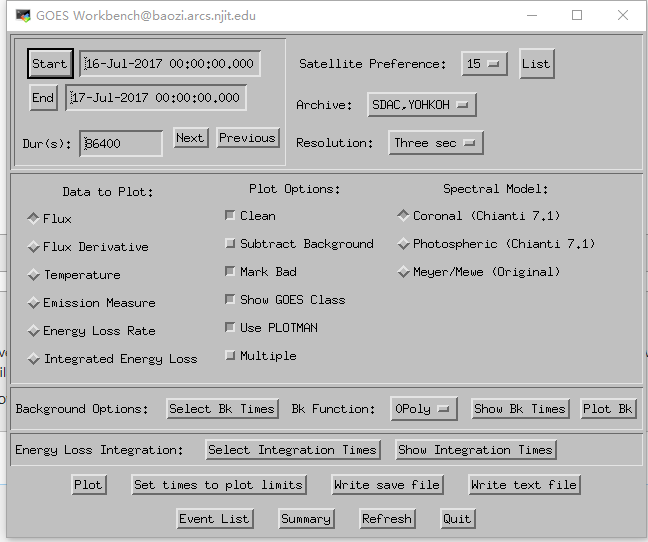
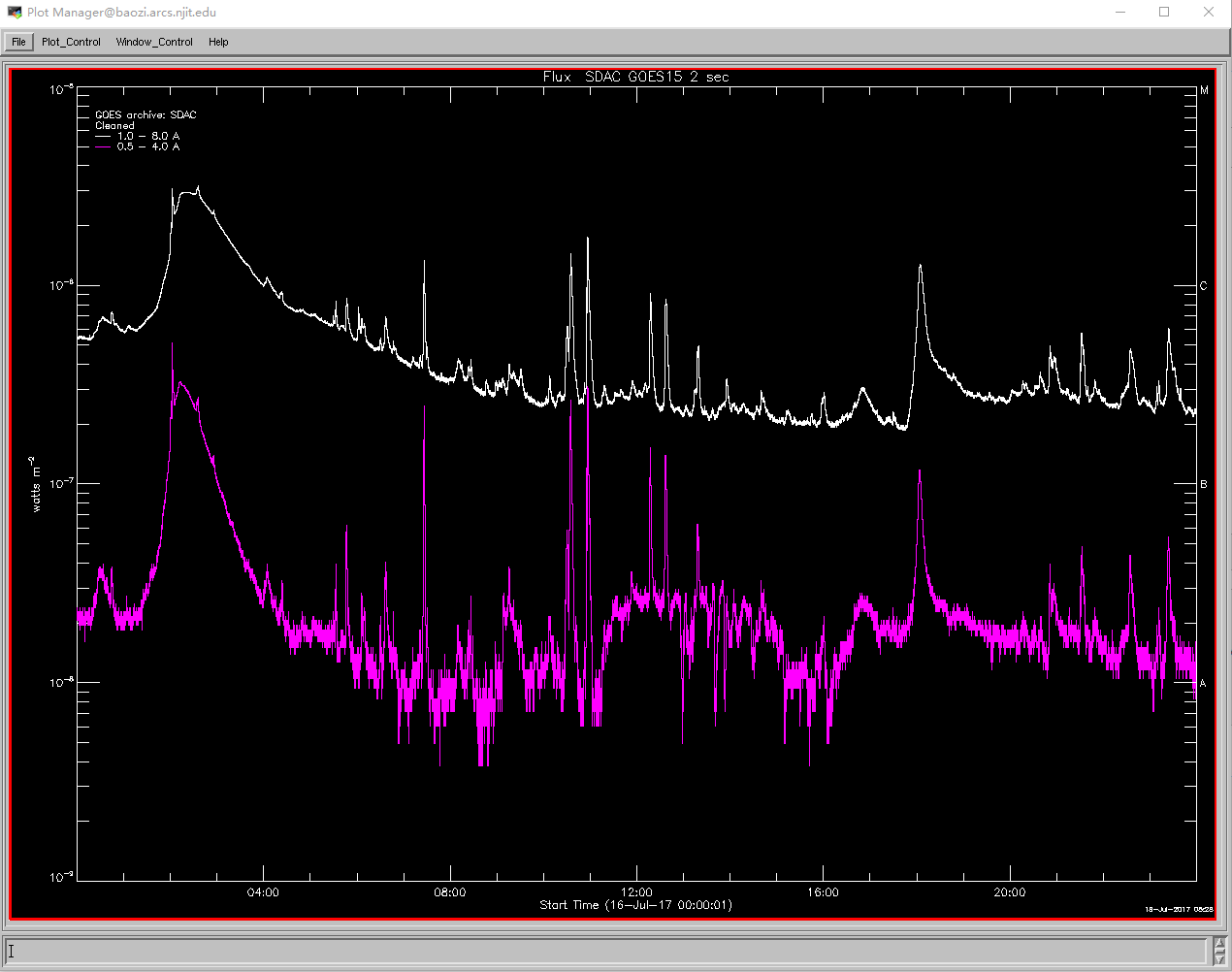
If you are in the server, you can do into idl to get the plot of Goes and RHESSI, which can help us identify the features in the dynamic spectrum.
Type 'goes' or 'hessi' you will see the command window.
Use Goes as a example, when you come into the command window, you can select parameters fot the plotting(mainly the timerange) and after clicking 'plot', you can control the plot in the menus and output the figure or you can directly write the idl savefile(for making the dynamic mivie later) in command window.
Always we need flux and derivate information for analysis.
Produce Detailed Dynamic Spectrum
Select the appropriate baselines
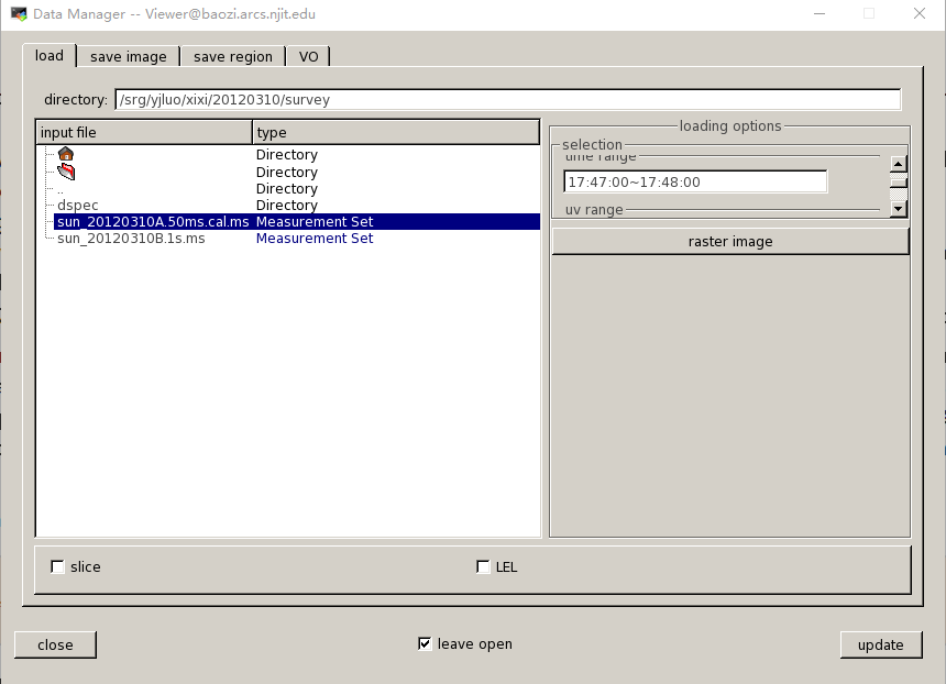
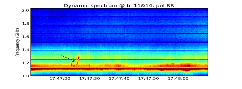
Usually we use the task 'dspec' to make the dynamic spectrum, use get_dspec to create a npz file, the most important input is timerange and baseline. You can use the casa task 'viewer' to check the visbility data( remember when using the viewer, don not select too long timerange).
When coming into the window of viewer. First in the data manager to select the timerange(no more than 20 minutes) and so on.
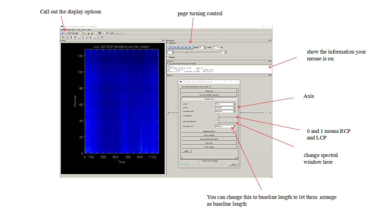
Then get into the display panel, set x,y,animation axis as 'time','channel'and'baselines'. Then you can check the display to select propriate baselines. Remember to check every spectral windows and both LCP and RCP.
Check Each baselines and better select both the longer baselines and shorter baselines to make the npz file.
Plot detailed dynamic spectrum
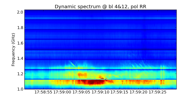
Use plt_dspec to do the plot, after getting the npz file, you can do the plot. Usually we are interested in both LCP and RCP, here set a example.
from suncasa.utils import dspec
msfile = 'sun_20120310A.50ms.ms' # the visbility data
vis = msfile
bl='4&12'
spw='0~7'
specfile = msfile+'.bl4-12.190000-194000.spec.npz'
timeran='17:58:50~17:59:30'
dspec.get_dspec(vis=vis,specfile=specfile,bl=bl,spw=spw,timeran=timeran)
dspec.plt_dspec(specfile=specfile,pol='RR',dmin=1,dmax=12)  #dmin and dmax is used to change color,pol can be selected as 'RR''LL'or'I'
To get the survey of the whole timerange, we need to get a movie, select the movie as True, you can get a folder called 'dspec' which including the figures to make the movie. You can also attach the goes savefile.
After getting the folders, you can use idl to create the movie like this 2012 Mar 10 event or directly use other ways.
Make overview radio/EUV image
Once you find something in the movie, you can back to the origrinal data to see the details, and we can use the calibrated data to make the overview image at that time.
Make radio image (clean)
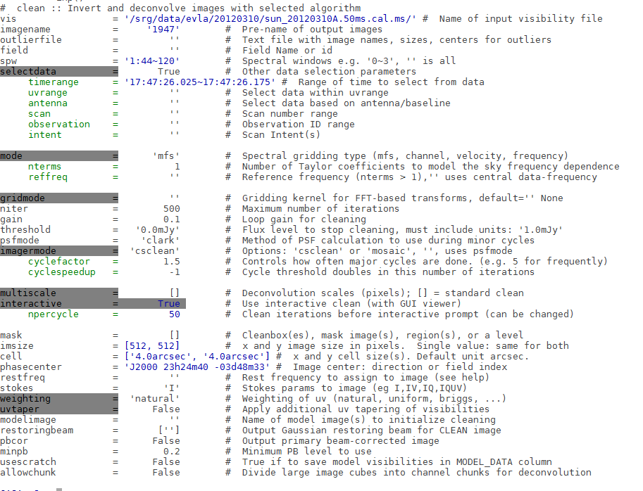
First step is to make the clean image using CASA task clean, you can also see details od clean in the CASA guide.
Select the appropriate parameters from the dynamic spectrum to do the clean.
Register cleaned CASA image into FITS file
Use the task 'helioimage2fits.imreg' to get the vla_fits file.
from suncasa.utils import helioimage2fits
vis='2110.50ms.cal.ms'
imagfile='2110.image' #clean image
timerange='21:10:31.275~21:10:31.675'
helioimage2fits.imreg(vis=vis,imagefile=imagefile,timerange=timerange)
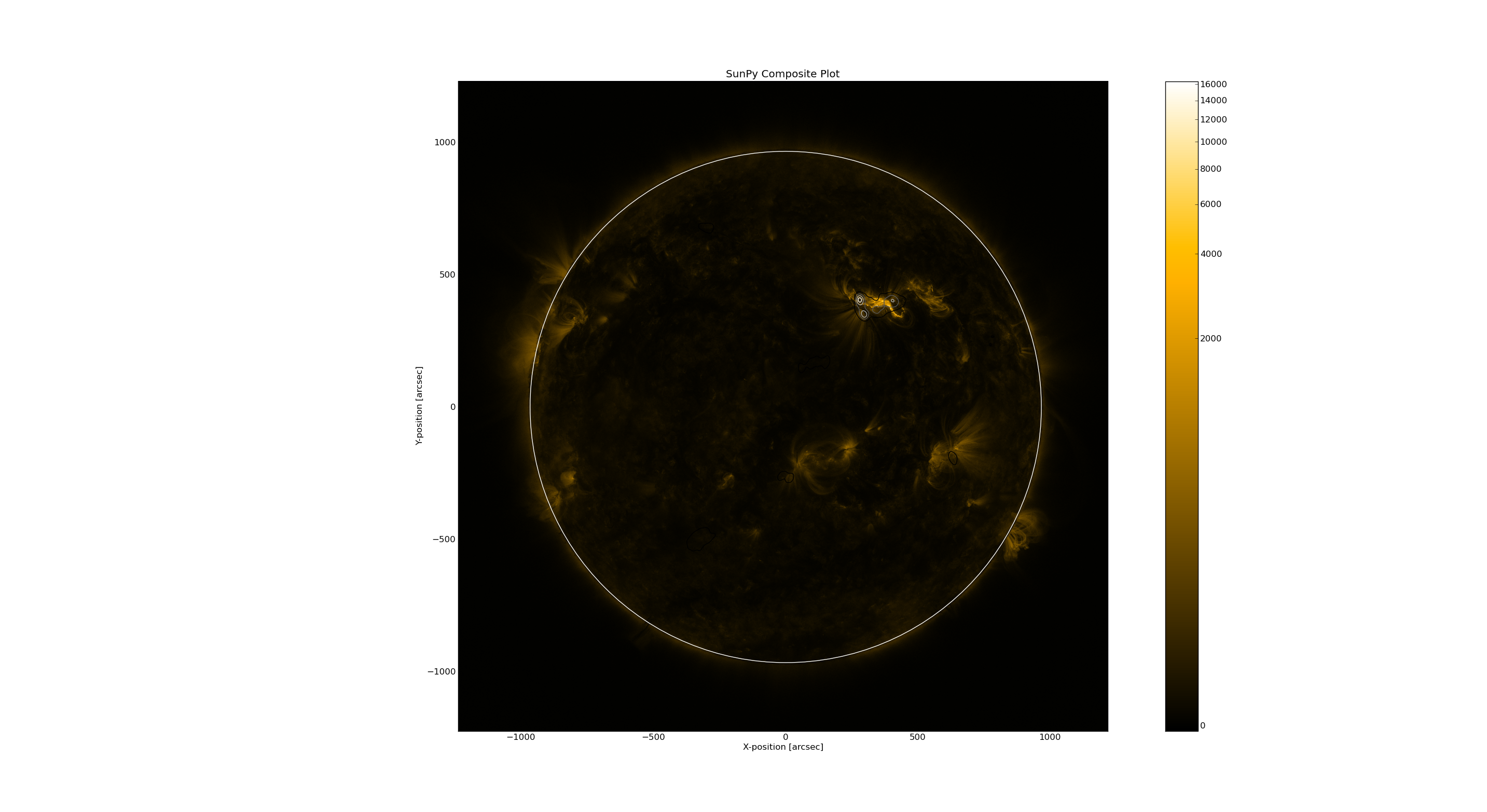
Plot radio image on AIA
Then add the vla-fits file into the aia map.
aiamap=smap.Map('aia_lev1_171a_2012_03_10t17_48_00_34z_image_lev1.fits')
vlafits='1747.fits'
vlamap=smap.Map(vlafits)
vlamap.data = vlamap.data.reshape(vlamap.meta['naxis1'],vlamap.meta['naxis2'])
cmap=smap.CompositeMap(aiamap)
cmap.add_map(vlamap,levels=np.array([0.5,0.7,0.9])*np.nanmax(vlamap.data))
cmap.peek()
You can also zoom in and out to see the details in the image.
