EOVSA Data Analysis Tutorial 2022
1. Introduction to EOVSA and Datasets
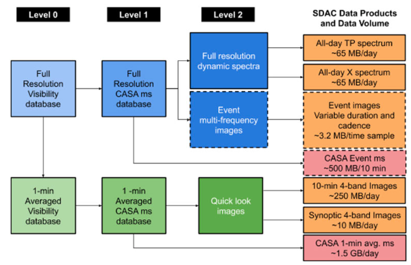
EOVSA (Expanded Owens Valley Solar Array) is a solar-dedicated radio interferometer operated by the New Jersey Institute of Technology. EOVSA observes the full disk of the Sun at all times when the Sun is >10 degrees above the local horizon, which is season dependent and ranges from 7-12 hours duration centered on 20 UT. Like any radio interferometer, the fundamental measurement for imaging is the correlated amplitude and phase between each pair of antennas, which is called a “complex visibility.” EOVSA’s 13 antennas form 78 such visibilities at any frequency and instant of time, i.e. 78 measurements of the spatial Fourier transform of the solar brightness distribution. EOVSA records these visibilities at 451 science frequency channels each second, in four polarization products (XX, YY, XY, YX), as well as additional total flux measurements from each individual antenna. These data are then processed through a pipeline processing system whose data flow is shown in the block diagram (Figure 1). One of the outputs of the pipeline is a visibility database in a widely used open-standard format called a CASA measurement set (or “ms”; CASA is the Common Astronomy Software Applications package used by many modern interferometer arrays).
EOVSA delivers the radio interferometry data on the following three levels:
- Level 0 - Raw visibility data - This includes observations of cosmic sources for phase calibration, and gain and pointing observations required for total power calibration.
- Level 1 - Calibrated visibility data - After applying calibration and other preliminary processing to level 0 data, we create the calibrated visibility data in CASA ms format (second column in Figure 1). These visibility data have all of the required content to produce Level 2 images and spectrogram data in standard FITS format. The following tutorial will guide you through how to make EOVSA images and spectrogram from visibility data. We provide a set of standard ms’s for each day (pink solid boxes in Figure 1) for users who wish to start with visibility data. You can retrieve EOVSA 1-min averaged visibility data in CASA ms format from this page. Full-resolution EOVSA visibility data in CASA ms format will be provided per request. Please contact the *EOVSA team if you wish to have Level 1 visibility data for a specific event.
- Level 2 - Images and spectrogram data in standard FITS format - Most users, however, will prefer to work with spectrogram (frequency-time) and image data, which are also outputs of the pipeline system shown in Figure 1 (orange boxes). Spectrograms are provided as standard FITS tables containing the frequency list, list of times, and data in both total power and a sum of amplitudes over intermediate-length baselines (cross power). Likewise, image data products are in FITS format with standard keywords and are converted into the Helioprojective Cartesian coordinate system compatible with the World Coordinate System (WCS) convention, along with correct registration for the spatial, spectral, and temporal coordinates. Both the spectrogram and image data products are calibrated and have physical radio intensity units (sfu for spectrograms and brightness temperature for radio images).
2. Browsing and Obtaining EOVSA data
EOVSA Browser
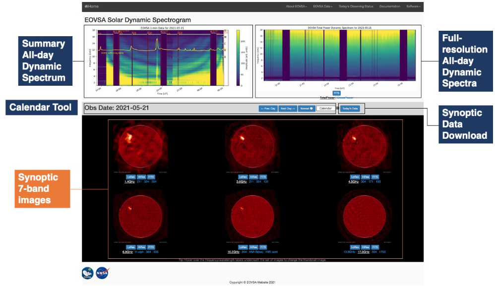
The most convenient way for browsing Level 2 EOVSA data is through the EOVSA Browser. The overview EOVSA dynamic spectra on the top-left panel are from the median of the uncalibrated cross-power visibilities at a few short baselines, which are not (but a good proxy of) the total-power dynamic spectra. The effects of spatial information blended in the cross-power visibilities can be clearly seen as the "U"-shaped features throughout the day, which are due to the movement of the Sun across the sky that effectively changes the length and orientation of the baselines. Flare emission can be seen in the dynamic spectra, which usually appears as vertical bright features across many frequency bands. The pipeline quicklook full-disk images are also displayed for the given frequencies along with multi-wavelength full-disk maps such as SDO AIA, HMI, BBSO H-alpha by hovering on the buttons on the bottom of each map.. More information can be found on this page. The figure on the right shows an example of the overview EOVSA dynamic spectrum for 2021 May 07.
RHESSI Browser
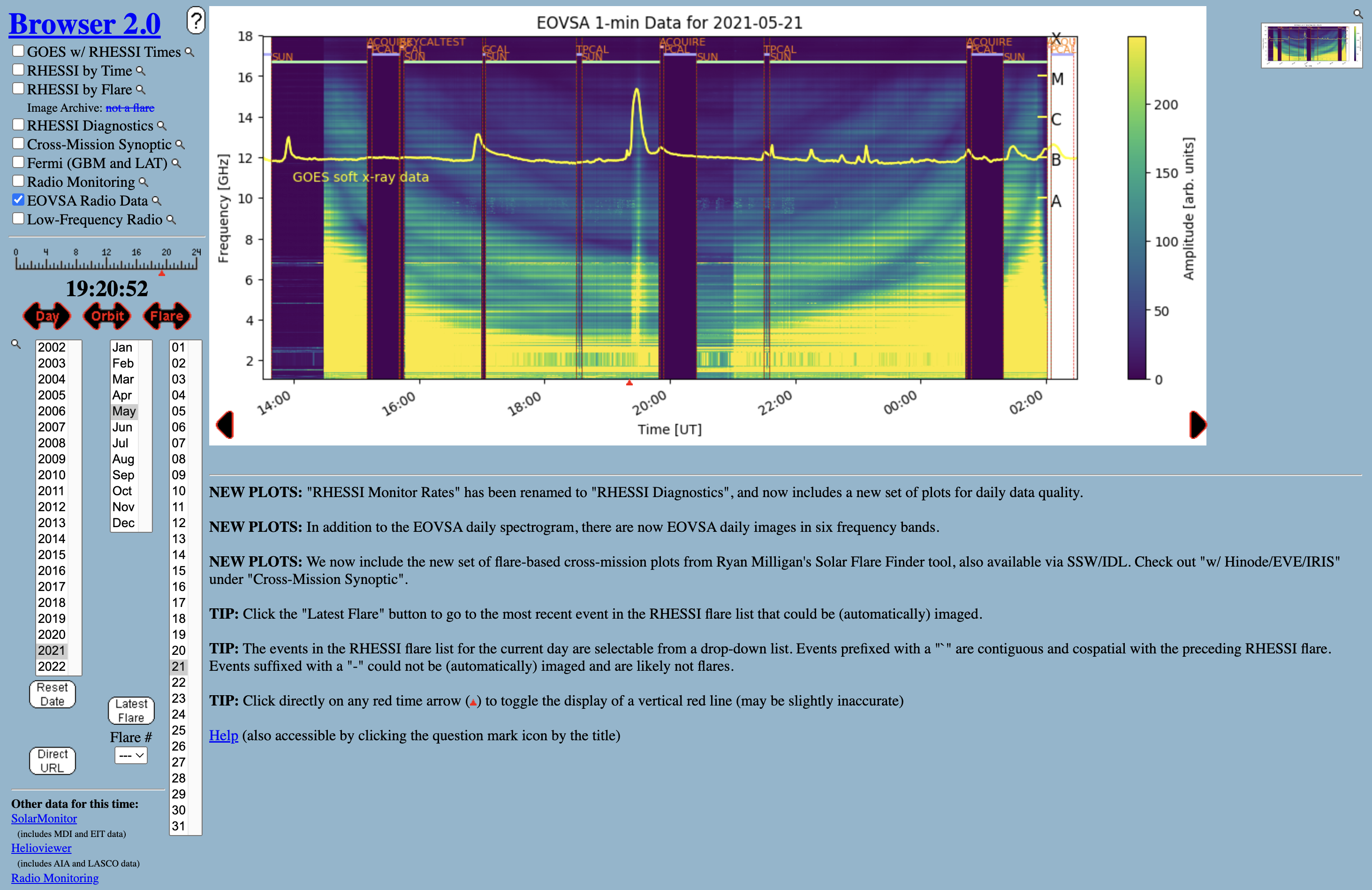
EOVSA data can also be browsed through RHESSI Browser. Check the "EOVSA Radio Data" box on the data selection area (top-left corner). Then select year/month/date to view the overall EOVSA dynamic spectrum. Note if a time is selected at early UTC hours (e.g., 0-3 UT), it will show the EOVSA dynamic spectrum from the previous day. Also, note that EOVSA data were not commissioned for spectroscopic imaging prior to April 2017.
Level 0 (raw visibility) Data
Once you identify the flare time, you can find the full-resolution (1-s cadence) uncalibrated visibility files (in Miriad format) at this link. Each data file is usually 10 minutes in duration. The name convention is YYYYMMDD (folder name) /IDBYYYYMMDDHHMMSS (file name), where the time in the file name indicates the start time of the visibility data. However, to be useful for imaging, these files must be first calibrated and then converted to a CASA measurement set. At present, this can only be done with software at the OVRO site although we are working on software to allow this processing to be done elsewhere. For now, please request this processing to be done for you by emailing Dale Gary, Bin Chen, Sijie Yu, or others you may know in the solar radio group.
Level 1 (calibrated visibility) Data
The images you see in the browser are generated by an automated pipeline that also produces calibrated CASA ms datasets, but at 1-min integration. If a 1-min cadence is sufficient for your purposes, you may wish to download the calibrated data and perform your own imaging. The 1-min cadence calibrated data are at this link. You should be aware that a model disk has been subtracted from the visibilities in these files, which is what you want if you are interested in imaging active regions or flares. It is possible to add the model back, but this is not available (yet) in standard software, so please contact someone in the NJIT solar radio group for help with that.
Other useful links
- EOVSA User Forum
- EOVSA Flare list
- EOVSA browser
- EOVSA wiki
- EOVSA 1-min averaged CASA ms database
- SunCASA on Github and PyPI
- Flare pipeline?
3. Software requirements and installation
EOVSA data processing and analysis are developed over two packages:
- SunCASA A Python wrapper around CASA (the Common Astronomy Software Applications package) for synthesis imaging and visualizing solar spectral imaging data. CASA is one of the leading software tools for "supporting the data post-processing needs of the next generation of radio astronomical telescopes such as ALMA and VLA", an international effort led by the National Radio Astronomy Observatory. The current version of CASA uses Python (3.6, 3.10*) interface. More information about CASA can be found on NRAO's CASA website . Note, CASA is available ONLY on UNIX-BASED PLATFORMS (and therefore, so is SunCASA).
- GSFIT A IDL-widget (GUI)-based spectral fitting package called GSFIT, which provides a user-friendly display of EOVSA image cubes and an interface to fast-fitting codes (via platform-dependent shared-object libraries).
For this tutorial, we will demonstrate using SunCASA to create EOVSA image and spectrogram from the visibility data observed for an M class flare on 2021 May 07. There are two approaches to accessing the SunCASA package:
- Through Google Colaboratory (colab) which hosts a free virtual environment that requires no setup and runs entirely in the cloud. For example, the EOVSA workspace of this tutorial explains the analysis setup.
- Install on your own machine, and run the notebook as a regular Jupyter Notebook. See SunCASA Installation section below, also this page and GSFIT Installation for instructions.
4. Download Sample EOVSA Data for the Tutorial
For this tutorial, we use an M4 class flare on 07 May 2021, around 19:00 UT occurred near the solar east limb as viewed from Earth, and was well observed by Solar Orbiter (including the STIX instrument). For other recent EOVSA events, check here. Here, we provide a calibrated and self-calibrated EOVSA visibility dataset in CASA ms format (IDB20210507_1840-1920XXYY.cal.10s.slfcaled.ms) which is ready for science analyses purposes,
5. Information on the EOVSA Visibility Data (CASA Measurement Set)
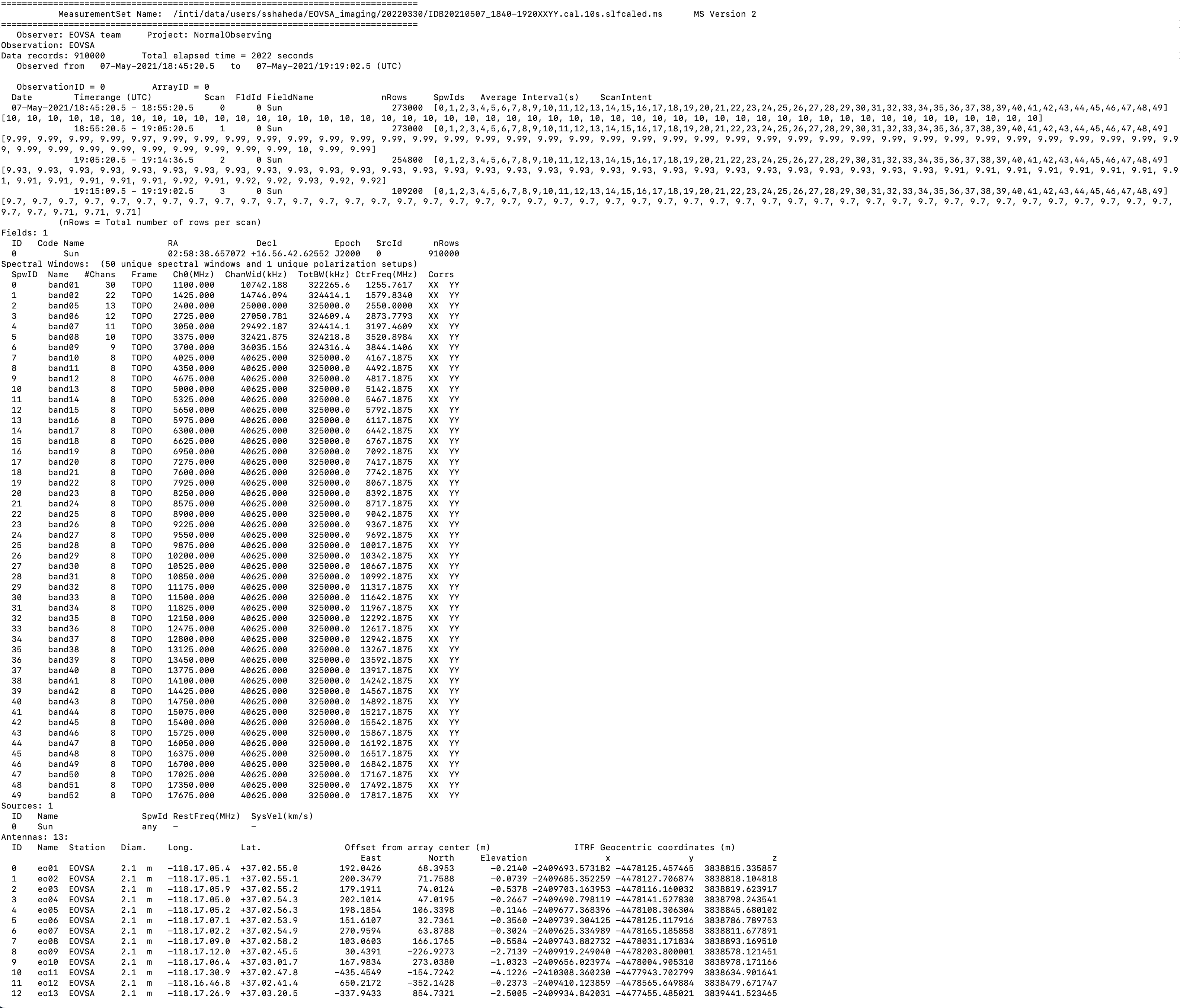
With the pip installation, the CASA modules may be used in a standard Python manner. For example, CASA tasks can be invoked using import, while CASA tools are Python classes that first need to be instantiated to create usable objects. A useful first task to run is listobs, which provides a summary of the measurement set.
## in SunCASA
from casatasks import listobs
import os
msfile = 'IDB20210507_1840-1920XXYY.cal.10s.slfcaled.ms'
rc = listobs(vis=msfile, listfile = msfile + '.listobs', overwrite=True)

print(os.popen("cat " + msfile + ".listobs").read())
6. Self-calibration (optional)
Self-calibration is often needed in bringing out details of the flare at multiple frequencies. An example script, run in SunCASA, for doing self-calibration of the 2017 Aug 21 flare at ~20:20 UT can be found at here. The EOVSA workspace discussed along with this tutorial anyway uses the self-calibrated dataset for analysis.
7. Cross-Power Dynamic Spectrum
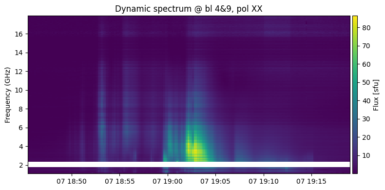
The first module we introduce is dspec. This module allows you to generate a cross-power dynamic spectrum from an MS file, and visualize it. You can select a subset of data by specifying a time range, spectral windows/channels, antenna baseline, or uvrange. The selection syntax follows the CASA convention. More information of CASA selection syntax may be found in the above links or the Measurement Selection Syntax.
## in SunCASA
from suncasa import dspec as ds
import time
           ## define the output filename of the dynamic spectrum
specfile = msfile + '.dspec.npz'
           ## The example below shows the cross-power spectrogram from a baseline selected using the parameter "bl".
           ## bl = '4&9' means selecting a baseline from Antenna ID 4 (Antenna Name "eo05") correlating with Antenna ID 9
           ## (Antenna Name "eo10") - refer listobs output.
           ## you can also use the "bl" parameter to select multiple baseline(s), i.e., bl='0&2;4&9;8&11'.

           ## Hover over "Dspec" in the next line to see additional arguments such as frequency range ("spw"), and time range ("timeran")
           ## or use help(ds.Dspec)
           ## this step generates a dynamic spectrum and saves it to specfile as a numpy .npz file
d = ds.Dspec(msfile, bl='4&9', specfile=specfile)
d.plot(vmin=None, vmax=None, pol='XX')
print(d.data.shape) # The shape gives the dimensions of polarization, baselines, frequencies, time
Alternative methods of using the "dspec" task are discussed in the EOVSA workspace.
NOTE: If you are using your own machine, the plotting should be in interactive mode. In that mode, hovering your mouse over the dynamic spectrum allows you to read the time, frequency, and flux information under the cursor at the bottom of the window.
8. Quick-Look Imaging
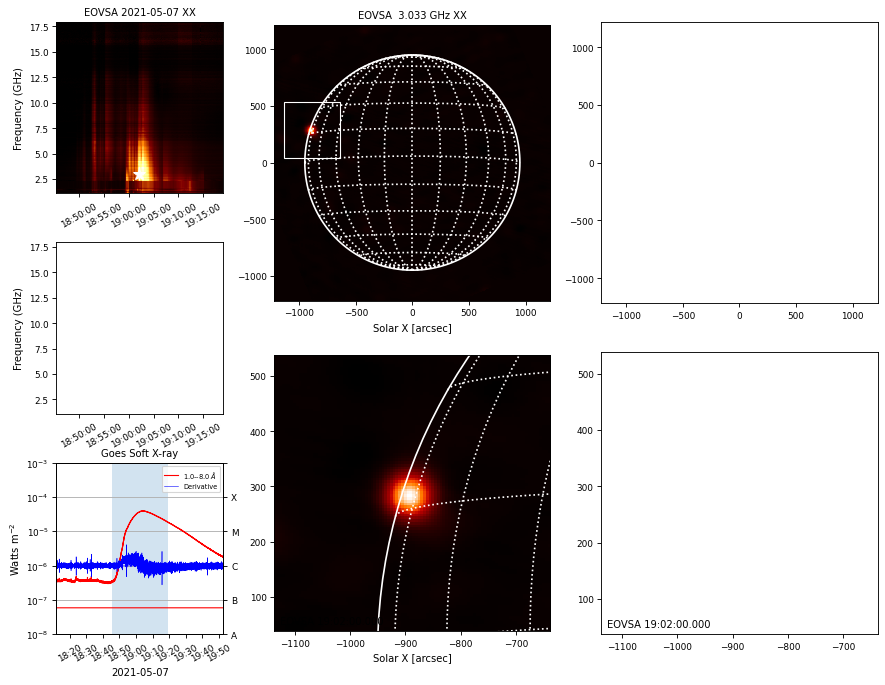
We use CASA's CLEAN algorithm for EOVSA imaging. As the default coordinate system is equatorial, solar coordinate transformation and image registration need to be done to place the image into the usual Helioprojective Cartesian Coordinates (X- and Y-axes are Solar X and Solar Y in arcsecond unit, respectively). We have bundled a number of these steps into a module named qlookplot, allowing users to generate an observing summary plot showing the cross power dynamic spectrum, GOES light curves and EOVSA quick-look images.
Now, let us start with making a summary plot of the EOVSA image at the spectral windows 2 to 5 (2.4–3.7 GHz).
## in SunCASA
from suncasa.utils import qlookplot as ql
           ## (Optional) Supply the npz file of the dynamic spectrum from previous step.
           ## If not provided, the program will generate a new one from the visibility.

timerange = '19:02:00~19:02:10' ## set the time interval
spw = '2~5'                     ## select frequency range
stokes = 'XX'                   ## select stokes XX
plotaia = False                 ## Initially, turn off AIA image plotting, default is True

ql.qlookplot(vis=msfile, specfile=specfile, timerange=timerange, spw=spw, \
    stokes=stokes, plotaia=plotaia, restoringbeam=['60arcsec'], robust=0.5)
The empty panels are there as only one polarization is selected for imaging/spectroscopy.
Feel free while working in EOVSA Workspace to explore by adjusting the above parameters, e.g. use a different time range ("timerange" parameter) and/or frequency range ("spw" parameter).
Quick-look Imaging with AIA data
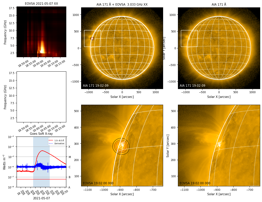
With qlookplot, it is easy to engage solar data from SDO/AIA in the summary plot. Setting plotaia=True in the qlookplot command will download SDO/AIA data at the given time to current directory and add it to the summary plot.
## in SunCASA
outfits = 'EOVSA_20210507T190205.000000.outim.image.fits'
ql.qlookplot(vis=msfile, specfile=specfile, timerange=timerange, spw=spw, \
    stokes=stokes, plotaia=True)
The resulting radio image is a 4-D datacube (in solar X-pos, Y-pos, frequency, and polarization), which is, by default, saved as a fits file Instrument_yymmddTHHMMS.ffffff.outim.image.fits under your working directory. An alternate name for the output fits file can be specified using the outfits parameter. In this example, we combine all selected frequencies (specified in keyword spw) into one image (i.e., multi-frequency synthesis). Therefore the third axis only has one plane. The fourth axis contains polarization. In this example, the fourth axis only has one plane as well (XX). Here is the relevant information (first few lines) in the header of the resulting FITS file.
In [1]: from astropy.io import fits
In [2]: hdu = fits.open('EOVSA_20210507T190230.000000.outim.image.fits')[0]
In [3]: hdu.header
Out[3]:
SIMPLE  =                    T / conforms to FITS standard
BITPIX  =                  -64 / array data type
NAXIS   =                    4 / number of array dimensions
NAXIS1  =                  512 / Nx
NAXIS2  =                  512 / Ny
NAXIS3  =                    1 / number of frequencies
NAXIS4  =                    1 / number of polarizations
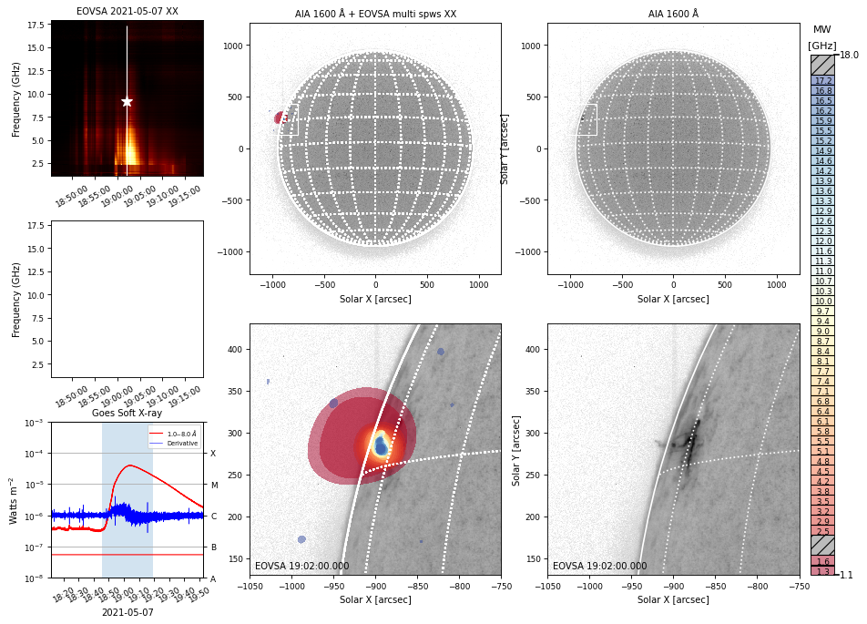
By default, qlookplot produces a full sun radio image (512x512 with a pixel size of 5"). If you know where the radio source is (e.g., from the previous full-Sun imaging), you can make a partial solar image around the source by specifying the image center (xycen), pixel scale (cell), and image field of view (fov). Here we show an example that images for each spectral window in this data set (from spw 0 to 49) at the same time interval around 19:02 UT. At high frequencies, the microwave source concentrates near the flare site, corresponding pretty well with the flare kernel in SDO/AIA. At low frequencies, the microwave source extends to higher altitudes in the corona. Again, feel free to change some of these parameters to explore what they do.
Quick-look Imaging with AIA data and all spw
Next, we will make images for every single spectral window in this data set (from spw 0 to 47).
## in SunCASA
from suncasa.utils.mstools import time2filename
timerange = '19:02:00~19:02:10'   ## set the time interval
spw = ['{}'.format(l) for l in range(48)].     ## select (almost) all spectral windows from spw id #0 to #47
outfits = time2filename(visibility_data,timerange=timerange)+'.outim.image.allbd.fits'

stokes = 'XX'.            ## select stokes XX
xycen = [-900, 280]       ## image center for clean in solar X-Y in arcsec
cell=['2.0arcsec']        ## pixel scale
imsize=[128]              ## number of pixels in X and Y. If only one value is provided, NX = NY
fov = [300,300]           ## field of view of the zoomed-in panels in unit of arcsec

plotaia = True            ## turn off AIA image plotting, default is True
aiawave = 1600            ## AIA passband in Å. The options are [171,131,304,335,211,193,94,1600,1700]
acmap = 'gray_r'          ## Choose the coloar map for AIA images. If not provided, the program will use default AIA colormap.

ql.qlookplot(vis=visibility_data, specfile=specfile, timerange=timerange,
             spw=spw, stokes=stokes, plotaia=plotaia, aiawave=aiawave,
             restoringbeam=['60arcsec'], robust = 0.5, acmap=acmap,
             imsize=imsize,cell=cell,xycen=xycen,fov=fov,
             outfits=outfits,overwrite=False)
9. Downloading fits files to your local system
This section is for interested users who wish to generate FITS files with full control of all parameters being used for synthesis imaging. Please follow the EOVSA Workspace for an example on downloading image fits files.
11. Spectral Fitting with GSFIT (optional)
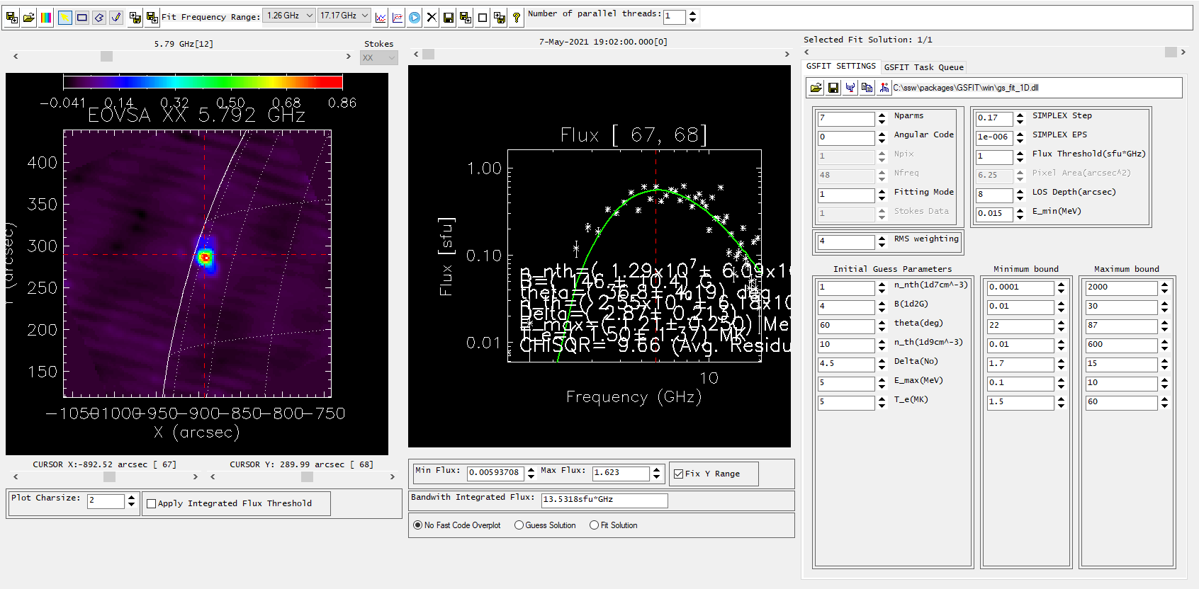
The .fits images obtained in the EOVSA Workspace can be read as an input to the GSFIT package. The screenshot of that is shown in Figure 9. Refer this page for a detailed description of further GSFIT analysis.
12. Installation of SunCASA (optional)
If you want to install SunCASA on your local machine follow this section. If not, run SunCASA directly on the Colab Workspace.
PIP wheels for SunCASA and its CASA dependencies are available as a Python 3 module from PyPI. This allows simple installation across most of the UNIX-BASED PLATFORMS (Linux & macOS) and import into standard *Python 3.6* environments. The RHEL 6/7 are the officially supported platforms for the casa modules. We have also tested the SunCASA/CASA packages under other Linux-based platforms such as Ubuntu 18, Scientific Linux 6/7, CentOS 7, as well as macOS Big Sur to some extent. YMMV for other versions of Linux or macOS. We do not recommend the use of Conda until CASA's compatibility with Conda is better understood.
Requirements
The following prerequisites must be present on the host machine before installing SunCASA:
- Python 3.6 (3.7 may also work, its compatibility with CASA is not fully understood yet)
- For Linux: libgfortran3 (yum or apt-get install)
- For MacOS: gcc (brew install, XQuartz and Xcode)
Installating SunCASA
Installation instructions are as follows (from a UNIX terminal window). First create a Python virtual environment named suncasaenv under the $HOME directory:
$ cd $HOME
$ python3.6 -m venv suncasaenv
NOTE: We strongly recommend using a Python virtual environment to prevent breaking any packages within a pre-existing Python environment.
Then use pip to install SunCASA within the newly-created virtual environment:
$ source suncasaenv/bin/activate
(suncasaenv) $ pip install --upgrade pip
(suncasaenv) $ pip install suncasa
NOTE: If this does not work, it could be due to unsuccessful installation of some dependencies. Running these commands should address this.
(suncasaenv) $ pip install casatasks
(suncasaenv) $ pip install casatools
(suncasaenv) $ pip install casadata
(suncasaenv) $ pip install PyQt5
(suncasaenv) $ pip install sunpy[all]
(suncasaenv) $ pip install suncasa
To exit the python venv, type "deactivate" from the terminal. However, the rest of this tutorial assumes the venv is active (to reactivate, type source $HOME/suncasaenv/bin/activate)
Updating a previous installation of SunCASA
You can update suncasa to its latest version by running:
(suncasaenv) $ pip install --upgrade suncasa
Sanity check
With the pip installation, SunCASA, as well as CASA, may be used in a standard Pythonic manner. For example, SunCASA modules and CASA tasks can be invoked using “import”, while CASA tools first need to be instantiated:
(suncasaenv) $ ipython
Python 3.6.9 (default, Jun 16 2021, 22:21:26)
Type 'copyright', 'credits' or 'license' for more information
IPython 7.16.1 -- An enhanced Interactive Python. Type '?' for help.
In [1]: import suncasa
In [2]: help(suncasa)
In [3]: import casatasks
In [4]: help(casatasks)
The use of python3 venv is a simple built-in method of containerizing the pip install such that multiple versions of SunCASA can be kept on a single machine in different environments. In addition, SunCASA is built and tested using standard (python 3.6) libraries which can be replicated with a fresh venv, keeping the libraries needed for SunCASA isolated from other libraries which may already be installed on your machine.

