EOVSA Imaging Workshop: Difference between revisions
| Line 6: | Line 6: | ||
Here are some basic information on CASA and software we developed to register the EOVSA CASA images: | Here are some basic information on CASA and software we developed to register the EOVSA CASA images: | ||
* [https://casaguides.nrao.edu CASA Guides] | |||
* [https://github.com/binchensun/suncasa suncasa] A CASA/python-based package being developed for imaging and visualizing spectral imaging data. A possibly useful (but perhaps buggy) routine ([https://github.com/binchensun/suncasa/blob/master/utils/helioimage2fits.py helioimage2fits.py]) is available for registering EOVSA/VLA (and possibly ALMA) CASA images. | |||
===Flare Data=== | ===Flare Data=== | ||
Revision as of 21:34, 2 January 2018
Sample EOVSA Data
To get started, we have made some calibrated flare and active region data in CASA measurement set format, available here. Here are some things to consider when working with the data:
- Antennas 1-8 and 12 have a wide sky coverage, while antennas 9-11 and 13 are the older equatorial mounts that can only cover +/- 55 degrees from the meridian. All antennas were tracking for the flare, but for portions of the all-day scan (roughly before 1600 UT or after 2400 UT) only 9 antennas will be tracking. Data for non-tracking antennas is NOT flagged, so if you try to image these periods, you'll need to manually omit ants 9-11 and 13.
- Because of the 2.5 GHz high-pass filters, data are taken only for bands 4-34. These will be labeled spectral window (spw) 0-31 in the measurement sets. However, band 4 (spw 0) is currently not calibrated, so only the 30 spectral windows 1-31 (bands 5-34, or frequencies 3-18 GHz) are valid data. You'll need to omit spw 0 when making images.
- In principle, circular polarization should be valid and meaningful, but no polarization calibration has been done (yet) so no non-ideal behavior (leakage terms, etc.) have been accounted for.
Here are some basic information on CASA and software we developed to register the EOVSA CASA images:
- CASA Guides
- suncasa A CASA/python-based package being developed for imaging and visualizing spectral imaging data. A possibly useful (but perhaps buggy) routine (helioimage2fits.py) is available for registering EOVSA/VLA (and possibly ALMA) CASA images.
Flare Data
Folder Flare_20170910 contains two measurement sets at full 1-s time resolution, each with 10-min duration:
- IDB20170910154625.corrected.ms (171 MB) [1] containing the first 10 minutes of the flare (15:46:25-15:56:25 UT), calibrated but no self-calibration
- IDB20170910154625.corrected.ms.xx.selfcaled (66 MB) [2] self-calibrated data for polarization XX
- IDB20170910155625.corrected.ms (232 MB) [3] containing the second 10 minutes of the flare (15:56:25-16:06:25 UT)
- IDB20170910155625.corrected.ms.xx.selfcaled (77 MB) [4] self-calibrated data for polarization XX
All Day Quiet Sun/Active Region Data
Folder AR_20170710 contains 8 calibrated measurements sets at 60-s time resolution.
- The seven UDB20170710*.corrected.ms are files for each scan separately, ranging in size from 7 - 150 MB depending on the length of the scan.
- UDB20170710_allday.ms (268 MB) [5] is the same data concatenated into a single file. However, each scan has a separate source ID.
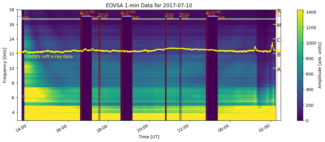
The AR data are also calibrated but not self-calibrated. In fact, we need to create a strategy for self-calibration of such data. You can get an overview of the AR coverage on that day by looking at the plot at http://ovsa.njit.edu/flaremon/daily/2017/XSP20170710.png. The separate scan files above are labeled with the time of the start of the scan, and each scan covers the time of continuous solar data between each calibration scan.
Possible Topics
Calibration
The (semi-)automatic calibrations we have done so far:
- Gain corrections: To account for changes of the attenuation settings (esp. during flares). See this page for details.
- Correcting for polarization mixing due to feed rotation: See this page for details.
- Antenna-based amplitude calibration: made by referencing total power and auto-correlation amplitudes to RSTN/Penticton total solar flux density measurements. See this page for details.
- Reference phase calibration: antenna-based, band-averaged phases derived from "reference" observations of strong celestial radio sources every night. See this page for details]
- Daily phase calibration: antenna-based multi-band delays resulted from the phase difference as a function from frequency between those derived from phase calibrators (usually observed 3 times during the day) and the reference calibrator. See this page for details.
More calibration being (or needs to be) developed:
- Polarization calibration: To calibrate absolute degree of circular polarization. Procedures need to be worked out.
- Per-channel bandpass (or single-band-delay) calibration within individual bands: To calibrate the phase/amplitude variations from channel to channel. Procedures need to be worked out.
Flare Imaging
Self-calibration Strategies
(Bin) Currently I am using a sliding window of five bands (band_to_selfcal +- 2 bands) to create a multi-frequency synthesized image as the input model for doing self-calibration at the band in question. Any alternative strategies? How about channel-by-channel selfcal?
Imaging Strategies
Clean? MEM? Optimum way to do spectral imaging? Here is an example made for the Sep 10 flare (Bin).
Quiet Sun and Active Region Imaging
Self-calibration Strategies
Imaging Strategies
Software Development
Currently we are using Python for analyzing calibration data and CASA for script-based imaging.
- What is the best approach to make an interactive imaging tool to serve the community (for both experts and non-experts)?
- How about the tool to visualize/analyze/make use of the resulted 4-D dynamic spectral imaging data?