Full Disk Simulations: Difference between revisions
| (22 intermediate revisions by 2 users not shown) | |||
| Line 7: | Line 7: | ||
= Creating Disk Models in CASA = | = Creating Disk Models in CASA = | ||
The first step in simulating a source is to create a "sky model," which is an image and associated descriptive header information to represent a source in the sky. CASA's [https://casaguides.nrao.edu/index.php/Simulation_Guide_Component_Lists_(CASA_5.4) componentlist] routines provide a recipe for creating different image components, including gaussian sources, point sources, disks, and so on. I created a python script diskmodel.py that eases the work of creating a disk model, which allows one to create a disk with unequal axes (generally larger in the equatorial axis and smaller in the polar axis). However, before it can be used one must have a good idea of the disk size and flux density of the disk. | The first step in simulating a source is to create a "sky model," which is an image and associated descriptive header information to represent a source in the sky. CASA's [https://casaguides.nrao.edu/index.php/Simulation_Guide_Component_Lists_(CASA_5.4) componentlist] routines provide a recipe for creating different image components, including gaussian sources, point sources, disks, and so on. I created a python script diskmodel.py that eases the work of creating a disk model, which allows one to create a disk with unequal axes (generally larger in the equatorial axis and smaller in the polar axis). However, before it can be used one must have a good idea of the disk size and flux density of the disk. | ||
| Line 20: | Line 19: | ||
9.24589, 10.24629, 11.24662, 12.24689, | 9.24589, 10.24629, 11.24662, 12.24689, | ||
13.24713, 14.24733, 15.24750]) | 13.24713, 14.24733, 15.24750]) | ||
which must correspond to the nearly periodic dips (nulls) in Figure 1. | which must correspond to the nearly periodic dips (nulls) in Figure 1. The value of <math>z</math> is related to the diameter of the solar disk by the relation | ||
<math>z = \pi D_{{\rm rad}} s_\lambda = \pi^2 D^{''}/(180\times3600) s_\lambda</math>, | |||
where <math>D_{{\rm rad}}</math> is the solar diameter in radians, <math>s_\lambda</math> is the uv distance in wavelengths, and the second relation is just the conversion to the solar diameter in arcsec, <math>D^{''}</math>. Note that the relevant disk size is not the photospheric radius, but rather the radius at radio frequencies, which varies with frequency and may even be different in the equatorial and polar axes. It may generally be expected to grow larger at lower frequencies, and grow more oblate near the equator as the coronal flux density becomes non-negligible. | |||
===Disk Fitting Python Code=== | |||
A set of three routines have been written in the Python module disk_fitting.py for the purposes of fitting the data in an all-day UDBms for the frequency-dependent disk shape and flux density. The input data are expected to be fully calibrated for amplitude and phase by the standard EOVSA pipeline. | |||
====read_ms()==== | |||
The routine read_ms() reads the UDBms visibilities and returns the relevant data in a convenient dictionary format that is used by the subsequent fitting routines. This routine must be used in the CASA (or SunCASA) environment. Here is an example: | |||
import disk_fitting as df | |||
vis = '/data1/eovsa/fits/UDBms/201908/UDB20190825.ms' | |||
out = df.read_ms(vis) | |||
It takes several minutes to read an entire day's file. | |||
====fit_diskmodel==== | |||
The routine fit_diskmodel() uses the output from read_ms() and fits a disk model for one band (or spectral window, spw, in CASA parlance) at a time. A nice summary plot of the data and fit is generated if doplot=True. One thing that the routine needs is the full Sun flux density spectrum derived from the RSTN fluxes collected each day by NOAA. The example below shows how to get that information and use it to fit a disk to the spw 40 data using fit_diskmodel(): | |||
import rstn | |||
from util import Time | |||
frq, flux = rstn.rd_rstnflux(t=Time('2019-09-01')) | |||
rstn_flux = rstn.rstn2ant(frq, flux, out['fghz']*1000, t=Time('2019-09-01')) | |||
fit_diskmodel(out, 40, rstn_flux, uvfitrange=[20,800], angle_tolerance=np.pi/2) | |||
The resulting plot is shown in Figure 2, where the uv range used for fitting (20-800 wavelengths) is shown by the blue-highlighted data points. One can see that the fit is excellent all the way out to 1000 wavelengths, and for this high frequency (14.7 GHz), the three fits (to equator, pole, and all points) all agree closely on the solar radius (964", 961", and 962", respectively). The photospheric disk is only 951" on this date, so these sizes are about 10" larger than the photosphere at this high frequency. The flux scale factor is also nominal, meaning that the RSTN flux density fits well to the data. [[file:20190901_band40_diskfit.png|thumb|right|300px|'''Fig. 2:''' Upper panel, fit of an Airy disk to baselines with more-or-less equatorial orientation. Middle panel, fit to baselines with more-or-less polar orientation. Lower panel, fit to all baselines.]] | |||
However, at lower frequencies things are a little more tricky. The plot in Figure 3 shows the spw 10 (5 GHz) fit for uv range 20-250 wavelengths. For that range, which covers the bulk of the flux, all of the disk sizes have increased quite a lot. In addition, the equatorial disk seems to be significantly larger than the polar disk, with an equatorial radius of 1045" and a polar radius of 1026". But also note how bad the fit becomes at longer uv distances. | |||
[[file:20190901_band10_diskfit1.png|thumb|right|300px|'''Fig. 3:''' Same as Figure 2, but for 5 GHz (spw 10), and fitting only the shorter baselines.]] | |||
When a larger uv range is used, as shown in Figure 4 (uvrange 200-900 wavelengths), a smaller disk size is suggested, around 990". This is still considerably larger than at spw 40. The true reason for the discrepancy in fits between Figures 3 and 4 is still being investigated. One idea is that there is a relatively sharp inner limb and a more gradual fall-off at greater heights. In this case, the longer baselines may resolve out this gradual decline and respond to the smaller, sharper limb, while the shorter baselines see the broader outer limb just fine. | |||
[[file:20190901_band10_diskfit2.png|thumb|right|300px|'''Fig. 4:''' Same as Figure 3, but fitting a wider range of baselines.]] | |||
====fit_vs_freq()==== | |||
The final routine, fit_vs_freq(), simply automates the running of fit_diskmodel() for all bands, plots the results, and returns the results in a nice summary dictionary. The syntax is a very simple one-line call: | |||
result = fit_vs_freq(out) | |||
The result dictionary has the following keys: | |||
'band' The spectral window band number from 0-49 | |||
'fghz' The frequency in GHz corresponding to the start of the band | |||
'eqradius' The equatorial radius for each band, in arcsec | |||
'polradius' The polar radius for each band, in arcsec | |||
'radius' The radius determined from the fit to all baselines | |||
'disk_flux' The flux density one should use in a later routine | |||
described below (this is 2 x RSTN) | |||
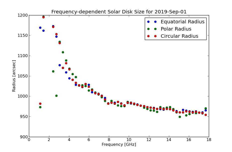
One should perhaps not take the summary plot results at face value in the light of Figures 3 and 4, however, since clearly different answers can be obtained depending on the uv range used for the fitting. Nevertheless, the results as a whole are plausible as shown in Figure 5. This plot is the result of one such run, where the uv fit range (internal to the fit_vs_freq() routine) is scaled outward in an algorithmic way according to | |||
uvfitrange = np.array([10,150])+np.array([1,18])*i | |||
where i is the band number. | |||
[[file:20190901_Solar_Disk_Size.png|thumb|right|300px|'''Fig. 5:''' Result of running fit_diskmodel() for all 50 spectral windows. There is a clear and plausible drop in solar radius with frequency.]] | |||
==Final Adopted Result of Fitting== | |||
In order to go further, a smooth fit (5th-order polynomial) to the red points has been done in order to create a frequency-dependent source model, described below. The following three input arrays, based on these fitting results, are used for creating the source model. | |||
* The list of spectral window starting frequencies, formatted for CASA: | |||
frq = np.array(['1.2624GHz', '1.5874GHz', '2.5625GHz', '2.8875GHz', '3.2125GHz', | |||
'3.5374GHz', '3.8624GHz', '4.1875GHz', '4.5125GHz', '4.8375GHz', | |||
'5.1625GHz', '5.4875GHz', '5.8125GHz', '6.1375GHz', '6.4625GHz', | |||
'6.7875GHz', '7.1125GHz', '7.4375GHz', '7.7625GHz', '8.0875GHz', | |||
'8.4124GHz', '8.7375GHz', '9.0625GHz', '9.3875GHz', '9.7125GHz', | |||
'10.037GHz', '10.361GHz', '10.687GHz', '11.011GHz', '11.337GHz', | |||
'11.662GHz', '11.986GHz', '12.312GHz', '12.636GHz', '12.962GHz', | |||
'13.287GHz', '13.611GHz', '13.937GHz', '14.261GHz', '14.587GHz', | |||
'14.912GHz', '15.236GHz', '15.562GHz', '15.886GHz', '16.212GHz', | |||
'16.536GHz', '16.862GHz', '17.187GHz', '17.511GHz', '17.836GHz'], | |||
dtype='|S9') | |||
* The flux density, in units of Jy, which are basically the RSTN sfu values doubled: | |||
fdens = np.array([ 891282, 954570, 1173229, 1245433, 1373730, 1506802, | |||
1613253, 1702751, 1800721, 1946756, 2096020, 2243951, | |||
2367362, 2525968, 2699795, 2861604, 3054829, 3220450, | |||
3404182, 3602625, 3794312, 3962926, 4164667, 4360683, | |||
4575677, 4767210, 4972824, 5211717, 5444632, 5648266, | |||
5926634, 6144249, 6339863, 6598018, 6802707, 7016012, | |||
7258929, 7454951, 7742816, 7948976, 8203206, 8411834, | |||
8656720, 8908130, 9087766, 9410760, 9571365, 9827078, | |||
10023598, 8896671]) | |||
* The solar disk size (assumed circular), formatted for CASA: | |||
dsize = np.array(['1228.0arcsec', '1194.0arcsec', '1165.0arcsec', '1139.0arcsec', '1117.0arcsec', | |||
'1097.0arcsec', '1080.0arcsec', '1065.0arcsec', '1053.0arcsec', '1042.0arcsec', '1033.0arcsec', | |||
'1025.0arcsec', '1018.0arcsec', '1012.0arcsec', | |||
'1008.0arcsec', '1003.0arcsec', '1000.0arcsec', '997.0arcsec', '994.0arcsec', '992.0arcsec', | |||
'990.0arcsec', '988.0arcsec', '986.0arcsec', '985.0arcsec', '983.0arcsec', '982.0arcsec', | |||
'980.0arcsec', '979.0arcsec', '978.0arcsec', '976.0arcsec', '975.0arcsec', '974.0arcsec', | |||
'972.0arcsec', '971.0arcsec', '970.0arcsec', '969.0arcsec', '968.0arcsec', '967.0arcsec', | |||
'966.0arcsec', '965.0arcsec', '964.0arcsec', '964.0arcsec', '963.0arcsec', '962.0arcsec', | |||
'962.0arcsec', '961.0arcsec', '960.0arcsec', '959.0arcsec', '957.0arcsec', '956.0arcsec']) | |||
==Using the Results to Create CASA Disk Model Images== | |||
CASA starts with properly formatted images from which to create uv models. I wrote a routine to create such properly formatted images in both FITS and CASA (.im) format. To make a frequency-dependent model, one must have such an image for each desired band (spw), which for EOVSA means 50 images. It is quite fast and easy to use the above three parameter arrays to create disk models, using the disk modeling routine diskmodel() that I wrote. The full call to create all 50 images is: | |||
for spw in range(50): | |||
diskmodel(outname='disk'+str(spw)+'_',direction='J2000 10h40m53.785s 08d20m37.60407s', | |||
reffreq=frq[spw],flux=fdens[spw],eqradius=dsize[spw],polradius=dsize[spw]) | |||
print spw | |||
where the loop over spectal window number calls diskmodel() to create .fits and .im files for each band. The diskmodel() routine assumes that the EOVSA bands are 325 MHz wide, and CASA requires that the reference frequency reffreq correspond to the center of the band. | |||
==Inserting the Model into the Observation Measurement Set== | |||
Once the model images are complete, they are inserted into the measurement set using the CASA 'ft' (Fourier Transform) task. The loop below accomplishes this for all 50 spw. | |||
import glob | |||
files = glob.glob('disk*.im') | |||
for i in range(50): | |||
# Find spw in filename (assumes filename 'disk<spw>_*.im') | |||
spw = int(files[i].split('disk')[1].split('_')[0]) | |||
ft(vis=vis, spw=str(spw), field='', model=str(files[i]), nterms=1, | |||
reffreq="''", complist="''", incremental=False, usescratch=True) | |||
This will result in filling the MODEL column of the dataset for each spw with the Fourier transform of the corresponding disk image. | |||
==Comparing Data and Model== | |||
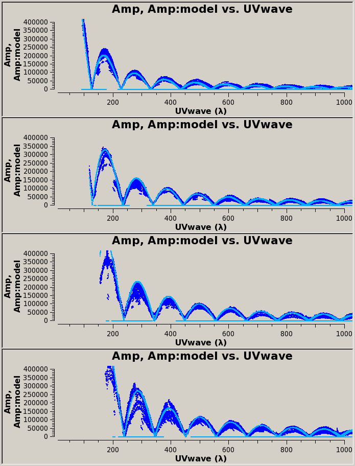
To check how well the disk models fit the data, it is useful to compare the data and model using plotms. The following commands will display the result in Figure 6. [[file:4band-comparison.png|thumb|right|300px|'''Fig. 6:''' Final comparison of MODEL data column (cyan) to the original DATA column (blue) for spectral windows 16, 26, 36, and 41.]] | |||
spws = ['16', '26', '36', '41'] | |||
for i in range(4): | |||
plotms(vis=vis, xaxis='uvwave', yaxis='amp', antenna='0~3', correlation='XX', | |||
gridrows=4, gridcols=1, ydatacolumn='data', rowindex=i, plotindex=2*i, | |||
plotrange=[10,1000,0,400000], clearplots=[True,False,False,False][i], spw=spws[i], | |||
customsymbol=True, symbolcolor='0000ff' , xsharedaxis=True) | |||
plotms(vis=vis, xaxis='uvwave', yaxis='amp', antenna='0~3', correlation='XX', | |||
timerange='14:00:00~23:00:00', | |||
gridrows=4, gridcols=1, ydatacolumn='model', rowindex=i, plotindex=2*i+1, | |||
plotrange=[10,1000,0,400000], clearplots=False, spw=spws[i], | |||
customsymbol=True, symbolcolor='00aaff' , xsharedaxis=True) | |||
Note that some amplitude scaling issues are apparent, so we should try amplitude selfcal to correct the data. | |||
The source code of the following procedures can be found in the [https://github.com/suncasa/suncasa/blob/master/eovsa/eovsa_diskmodel.py suncasa] package. | |||
Latest revision as of 20:10, 11 September 2019
Purpose
EOVSA's 13 antennas provide limited uv coverage for imaging the solar disk, but the baselines do contain considerable flux, especially on shorter baselines. We have good evidence that weak features of the quiet Sun (e.g. filament channels, prominences, and weak plage areas) do show up in the data, but the variations in brightness due to the poorly sampled disk often swamp them. The correct approach to imaging such features is to model the quiet solar disk and remove it from the uv data. then clean the residual flux that contains these weaker features, and finally add the disk model back. Self calibration also requires a good source model that includes the disk.
The purpose of this page is to describe the nuts and bolts of that procedure and document the performance.
NB: Since we are just getting started with this procedure, this page will initially present a number of tests. Ultimately it should become a definitive description of the procedure without a lot of false starts.
Creating Disk Models in CASA
The first step in simulating a source is to create a "sky model," which is an image and associated descriptive header information to represent a source in the sky. CASA's componentlist routines provide a recipe for creating different image components, including gaussian sources, point sources, disks, and so on. I created a python script diskmodel.py that eases the work of creating a disk model, which allows one to create a disk with unequal axes (generally larger in the equatorial axis and smaller in the polar axis). However, before it can be used one must have a good idea of the disk size and flux density of the disk.
Estimating disk axes and flux density from the data
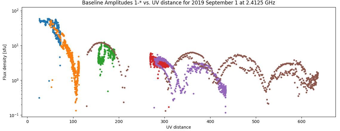
One can use the data themselves to estimate the size of the disk needed to fit the data. As it turns out, EOVSA visibilities provide excellent measures of the disk shape and flux density if we can make use of it. After a lot of effort, I believe we have an understanding of how to interpret the EOVSA visibilities in terms of the disk shape and flux density, and therefore how to fit the data to derive estimates for the three key parameters: equatorial radius, polar radius, and flux density. In practice, the flux density seems to fit quite well with the flux density imposed by the total power/auto-correlation calibration, so it is likely that we will do better just using the nominal flux density imposed from RSTN. Figure 1 shows an example of some data for 2019 Sep 01.
The visibilities due to the solar disk are the same as the Fourier Transform of a circular aperture, which is an Airy pattern (not an Airy function, which apparently is a different mathematical function). The power distribution vs. radius in an Airy disk is , where is the first-order Bessel function and is the peak intensity. However, in the uv-plane we are looking not at the power, but rather the electric field pattern itself, hence we are interested in the square root of this function, i.e. . Note that the first 15 zeros of the airy disk are listed as:
m = array([  1.21967,   2.23313,   3.23831,   4.24106,
             5.24276,   6.24392,   7.24476,   8.24539,
             9.24589,  10.24629,  11.24662,  12.24689,
            13.24713,  14.24733,  15.24750])
which must correspond to the nearly periodic dips (nulls) in Figure 1. The value of is related to the diameter of the solar disk by the relation
,
where is the solar diameter in radians, is the uv distance in wavelengths, and the second relation is just the conversion to the solar diameter in arcsec, . Note that the relevant disk size is not the photospheric radius, but rather the radius at radio frequencies, which varies with frequency and may even be different in the equatorial and polar axes. It may generally be expected to grow larger at lower frequencies, and grow more oblate near the equator as the coronal flux density becomes non-negligible.
Disk Fitting Python Code
A set of three routines have been written in the Python module disk_fitting.py for the purposes of fitting the data in an all-day UDBms for the frequency-dependent disk shape and flux density. The input data are expected to be fully calibrated for amplitude and phase by the standard EOVSA pipeline.
read_ms()
The routine read_ms() reads the UDBms visibilities and returns the relevant data in a convenient dictionary format that is used by the subsequent fitting routines. This routine must be used in the CASA (or SunCASA) environment. Here is an example:
import disk_fitting as df
vis = '/data1/eovsa/fits/UDBms/201908/UDB20190825.ms'
out = df.read_ms(vis)
It takes several minutes to read an entire day's file.
fit_diskmodel
The routine fit_diskmodel() uses the output from read_ms() and fits a disk model for one band (or spectral window, spw, in CASA parlance) at a time. A nice summary plot of the data and fit is generated if doplot=True. One thing that the routine needs is the full Sun flux density spectrum derived from the RSTN fluxes collected each day by NOAA. The example below shows how to get that information and use it to fit a disk to the spw 40 data using fit_diskmodel():
import rstn
from util import Time
frq, flux = rstn.rd_rstnflux(t=Time('2019-09-01'))
rstn_flux = rstn.rstn2ant(frq, flux, out['fghz']*1000, t=Time('2019-09-01'))
fit_diskmodel(out, 40, rstn_flux, uvfitrange=[20,800], angle_tolerance=np.pi/2)
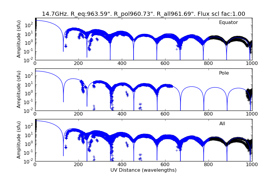
The resulting plot is shown in Figure 2, where the uv range used for fitting (20-800 wavelengths) is shown by the blue-highlighted data points. One can see that the fit is excellent all the way out to 1000 wavelengths, and for this high frequency (14.7 GHz), the three fits (to equator, pole, and all points) all agree closely on the solar radius (964", 961", and 962", respectively). The photospheric disk is only 951" on this date, so these sizes are about 10" larger than the photosphere at this high frequency. The flux scale factor is also nominal, meaning that the RSTN flux density fits well to the data.
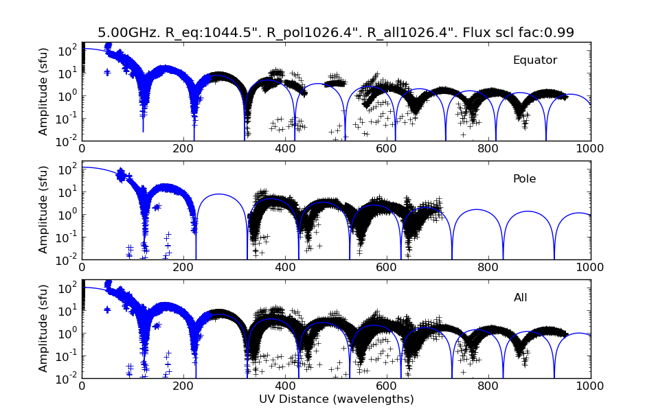
However, at lower frequencies things are a little more tricky. The plot in Figure 3 shows the spw 10 (5 GHz) fit for uv range 20-250 wavelengths. For that range, which covers the bulk of the flux, all of the disk sizes have increased quite a lot. In addition, the equatorial disk seems to be significantly larger than the polar disk, with an equatorial radius of 1045" and a polar radius of 1026". But also note how bad the fit becomes at longer uv distances.
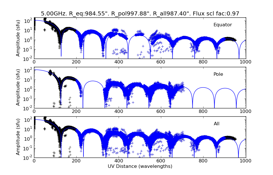
When a larger uv range is used, as shown in Figure 4 (uvrange 200-900 wavelengths), a smaller disk size is suggested, around 990". This is still considerably larger than at spw 40. The true reason for the discrepancy in fits between Figures 3 and 4 is still being investigated. One idea is that there is a relatively sharp inner limb and a more gradual fall-off at greater heights. In this case, the longer baselines may resolve out this gradual decline and respond to the smaller, sharper limb, while the shorter baselines see the broader outer limb just fine.
fit_vs_freq()
The final routine, fit_vs_freq(), simply automates the running of fit_diskmodel() for all bands, plots the results, and returns the results in a nice summary dictionary. The syntax is a very simple one-line call:
result = fit_vs_freq(out)
The result dictionary has the following keys:
'band'        The spectral window band number from 0-49
'fghz'        The frequency in GHz corresponding to the start of the band
'eqradius'    The equatorial radius for each band, in arcsec
'polradius'   The polar radius for each band, in arcsec
'radius'      The radius determined from the fit to all baselines
'disk_flux'   The flux density one should use in a later routine
                described below (this is 2 x RSTN)
One should perhaps not take the summary plot results at face value in the light of Figures 3 and 4, however, since clearly different answers can be obtained depending on the uv range used for the fitting. Nevertheless, the results as a whole are plausible as shown in Figure 5. This plot is the result of one such run, where the uv fit range (internal to the fit_vs_freq() routine) is scaled outward in an algorithmic way according to
uvfitrange = np.array([10,150])+np.array([1,18])*i
where i is the band number.
Final Adopted Result of Fitting
In order to go further, a smooth fit (5th-order polynomial) to the red points has been done in order to create a frequency-dependent source model, described below. The following three input arrays, based on these fitting results, are used for creating the source model.
- The list of spectral window starting frequencies, formatted for CASA:
frq = np.array(['1.2624GHz', '1.5874GHz', '2.5625GHz', '2.8875GHz', '3.2125GHz',
      '3.5374GHz', '3.8624GHz', '4.1875GHz', '4.5125GHz', '4.8375GHz',
      '5.1625GHz', '5.4875GHz', '5.8125GHz', '6.1375GHz', '6.4625GHz',
      '6.7875GHz', '7.1125GHz', '7.4375GHz', '7.7625GHz', '8.0875GHz',
      '8.4124GHz', '8.7375GHz', '9.0625GHz', '9.3875GHz', '9.7125GHz',
      '10.037GHz', '10.361GHz', '10.687GHz', '11.011GHz', '11.337GHz',
      '11.662GHz', '11.986GHz', '12.312GHz', '12.636GHz', '12.962GHz',
      '13.287GHz', '13.611GHz', '13.937GHz', '14.261GHz', '14.587GHz',
      '14.912GHz', '15.236GHz', '15.562GHz', '15.886GHz', '16.212GHz',
      '16.536GHz', '16.862GHz', '17.187GHz', '17.511GHz', '17.836GHz'],
     dtype='|S9')
- The flux density, in units of Jy, which are basically the RSTN sfu values doubled:
fdens = np.array([  891282,   954570,  1173229,  1245433,  1373730,  1506802,
       1613253,  1702751,  1800721,  1946756,  2096020,  2243951,
       2367362,  2525968,  2699795,  2861604,  3054829,  3220450,
       3404182,  3602625,  3794312,  3962926,  4164667,  4360683,
       4575677,  4767210,  4972824,  5211717,  5444632,  5648266,
       5926634,  6144249,  6339863,  6598018,  6802707,  7016012,
       7258929,  7454951,  7742816,  7948976,  8203206,  8411834,
       8656720,  8908130,  9087766,  9410760,  9571365,  9827078,
      10023598,  8896671])
- The solar disk size (assumed circular), formatted for CASA:
dsize = np.array(['1228.0arcsec', '1194.0arcsec', '1165.0arcsec', '1139.0arcsec', '1117.0arcsec',
'1097.0arcsec', '1080.0arcsec', '1065.0arcsec', '1053.0arcsec', '1042.0arcsec', '1033.0arcsec',
'1025.0arcsec', '1018.0arcsec', '1012.0arcsec',
'1008.0arcsec', '1003.0arcsec', '1000.0arcsec', '997.0arcsec', '994.0arcsec', '992.0arcsec',
'990.0arcsec', '988.0arcsec', '986.0arcsec', '985.0arcsec', '983.0arcsec', '982.0arcsec',
'980.0arcsec', '979.0arcsec', '978.0arcsec', '976.0arcsec', '975.0arcsec', '974.0arcsec',
'972.0arcsec', '971.0arcsec', '970.0arcsec', '969.0arcsec', '968.0arcsec', '967.0arcsec',
'966.0arcsec', '965.0arcsec', '964.0arcsec', '964.0arcsec', '963.0arcsec', '962.0arcsec',
'962.0arcsec', '961.0arcsec', '960.0arcsec', '959.0arcsec', '957.0arcsec', '956.0arcsec'])
Using the Results to Create CASA Disk Model Images
CASA starts with properly formatted images from which to create uv models. I wrote a routine to create such properly formatted images in both FITS and CASA (.im) format. To make a frequency-dependent model, one must have such an image for each desired band (spw), which for EOVSA means 50 images. It is quite fast and easy to use the above three parameter arrays to create disk models, using the disk modeling routine diskmodel() that I wrote. The full call to create all 50 images is:
for spw in range(50):
   diskmodel(outname='disk'+str(spw)+'_',direction='J2000 10h40m53.785s 08d20m37.60407s',
             reffreq=frq[spw],flux=fdens[spw],eqradius=dsize[spw],polradius=dsize[spw])
   print spw
where the loop over spectal window number calls diskmodel() to create .fits and .im files for each band. The diskmodel() routine assumes that the EOVSA bands are 325 MHz wide, and CASA requires that the reference frequency reffreq correspond to the center of the band.
Inserting the Model into the Observation Measurement Set
Once the model images are complete, they are inserted into the measurement set using the CASA 'ft' (Fourier Transform) task. The loop below accomplishes this for all 50 spw.
import glob
files = glob.glob('disk*.im')
for i in range(50):
    # Find spw in filename (assumes filename 'disk<spw>_*.im')
    spw = int(files[i].split('disk')[1].split('_')[0])
    ft(vis=vis, spw=str(spw), field=, model=str(files[i]), nterms=1,
       reffreq="", complist="", incremental=False, usescratch=True)
This will result in filling the MODEL column of the dataset for each spw with the Fourier transform of the corresponding disk image.
Comparing Data and Model
To check how well the disk models fit the data, it is useful to compare the data and model using plotms. The following commands will display the result in Figure 6.
spws = ['16', '26', '36', '41']
for i in range(4):
    plotms(vis=vis, xaxis='uvwave', yaxis='amp', antenna='0~3', correlation='XX',
           gridrows=4, gridcols=1, ydatacolumn='data', rowindex=i, plotindex=2*i,
           plotrange=[10,1000,0,400000], clearplots=[True,False,False,False][i], spw=spws[i],
           customsymbol=True, symbolcolor='0000ff' , xsharedaxis=True)
    plotms(vis=vis, xaxis='uvwave', yaxis='amp', antenna='0~3', correlation='XX',
           timerange='14:00:00~23:00:00',
           gridrows=4, gridcols=1, ydatacolumn='model', rowindex=i, plotindex=2*i+1,
           plotrange=[10,1000,0,400000], clearplots=False, spw=spws[i],
           customsymbol=True, symbolcolor='00aaff' , xsharedaxis=True)
Note that some amplitude scaling issues are apparent, so we should try amplitude selfcal to correct the data.
The source code of the following procedures can be found in the suncasa package.
