VLA Data Survey
List of Jansky VLA Solar Observations
| Date | VLA Time | Observing Setup | Context | Details | Flare Events | RHESSI | Fermi/GBM | Publications |
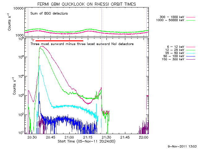
| Nov 5, 2011 | 20:39:08-23:07:56 | 17 ants in Config D 1-2 GHz/1 MHz, 0.1 s |
Overview dynamic spectrum summary |
VLA_20111105 | M1.8@20:37 | Yes; 12-25 | Yes; 50-100 | Chen+, ApJL, 2013 |
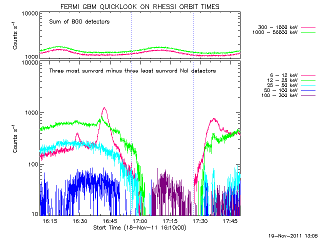
| Nov 18, 2011 | 17:02:17-17:25:50 | 17 ants in Config D 1-2 GHz/1 MHz, 0.1 s |
Overview dynamic spectrum summary |
VLA_20111118 | C2.7@17:25 | Yes; 6-12 | Yes; 12-25 | |
| Feb 25, 2012 | 17:04:00-17:40:17 | 26 ants in Config C | -- | 20 dB attn delay calibration | -- | -- | -- | |
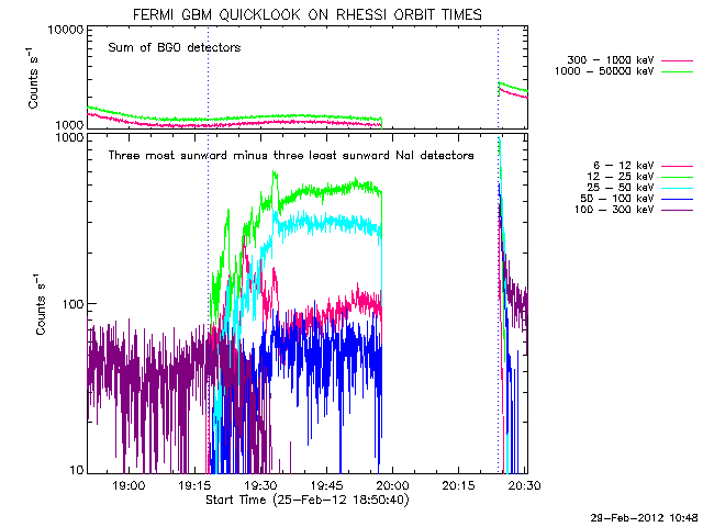
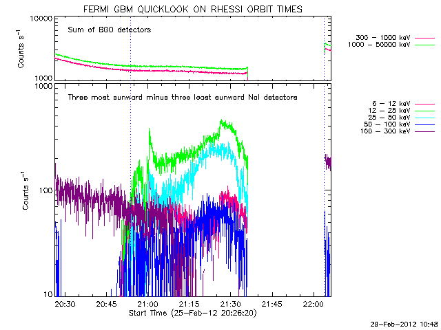
| 18:00:06-22:17:00 | 26 ants in Config C 1-2 GHz/1 MHz, 1s |
Overview dynamic spectrum summary |
VLA_20120225 | B3.6 microflare @19:29 | No | Yes; 6-12 | ||
| B4.0 microflare @20:50 | Yes; 6-12 | Yes; 25-50 | Sharma+ in prep | |||||
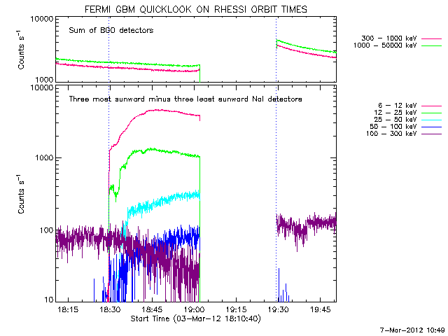
| Mar 3, 2012 | 17:53:23-21:44:54 | 15 ants in Config C 1-2 GHz/1 MHz, 50 ms |
Overview dynamic spectrum summary |
VLA_20120303 | C1.9@18:13 | Yes; 12-25 | Yes; 12-25 | Chen+, ApJ, 2014, Chen+, Science, 2015, Wang+, ApJ, 2017 |
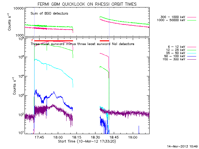
| Mar 10, 2012 | 17:46:18-21:46:46 | 15 ants in Config C 1-2 GHz/1 MHz, 50 ms |
Overview dynamic spectrum summary |
VLA_20120310 | M8.4@17:40 | Yes; 25-50 | Yes; 50-100 | Luo+ in prep, Zhang+ in prep |
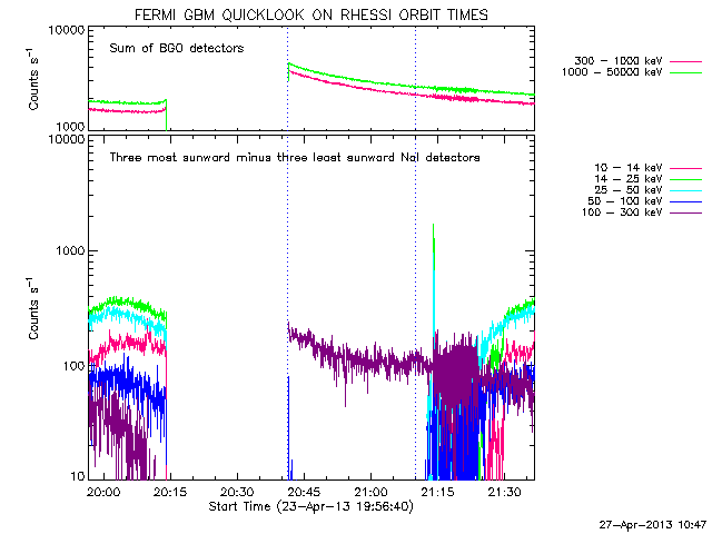
| Apr 23, 2013 | 19:37:36-21:32:12 | 13 ants in Config D L:1-2 GHz/2 MHz, 50 ms S: 2-4 GHz/2 MHz, 50 ms |
Overview dynamic spectrum summary |
VLA_20130423 | C1.8@20:34:10 | Yes; 12-25 | No | |
| B?@20:36 | Yes; 12-25 | No | Battaglia+ in prep | |||||
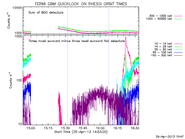
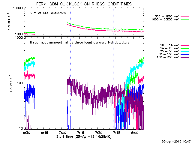
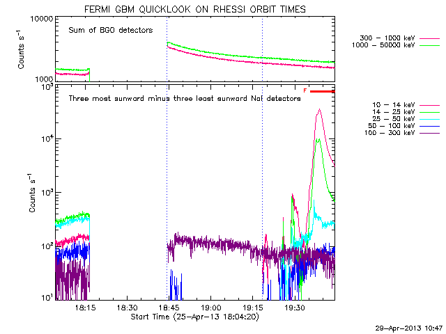
| Apr 25, 2013 | 14:36:10-19:03:52 | 13 ants in Config D L:1-2 GHz/2 MHz, 50 ms S: 2-4 GHz/2 MHz, 50 ms |
Overview dynamic spectrum summary |
VLA_20130425 | C1.0@15.31 | Yes; 6-12 | No | |
| C1.5@16:23 | Yes; 12-25 | Yes; 14-25 | ||||||
| C3.9@17:17 | Yes; 12-25 | No | ||||||
| C5.6@17:28 | Yes; 12-25 | No | ||||||
| C1.3@18:28 | Yes; 12-25 | No | ||||||
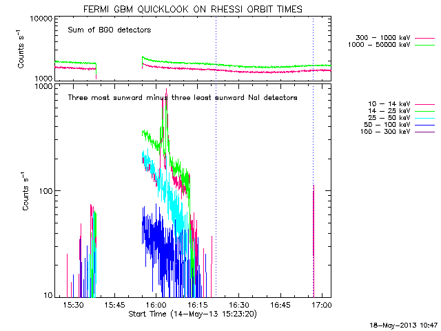
| May 14, 2013 | 14:38:36-17:35:13 | 13 ants in Config D L:1-2 GHz/2 MHz, 50 ms S: 2-4 GHz/2 MHz, 50 ms |
Overview dynamic spectrum [summary] |
VLA_20130614 | C1@15:37:08 | Yes; 6-12 | Yes; 14-25 | |
| C1@16:04:13 | ||||||||
| C1@16:24:03 | ||||||||
| C1@16:56:39 | ||||||||
| Jun 10, 2013 | 15:57:34-18:34:31 | 27 ants in Config D L,S,C/1 MHz, 1 s |
-- | 20 dB attn delay calibration | -- | -- | -- | |
| Aug 1, 2013 | 14:55:28-15:32:29 | 27 ants in Config D L,S,C/1 MHz, 1 s |
-- | 20 dB attn delay calibration | -- | -- | -- | |
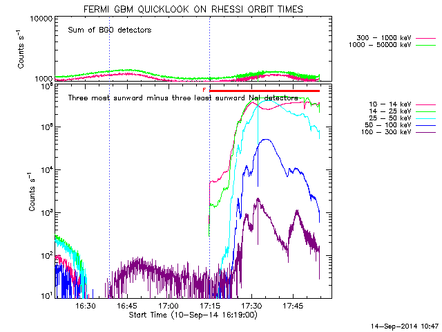
| Sep 10, 2014 | 21:14:56-22:57:52 | 27 ants in Config D C: 4.2-5.2, 7-8 GHz/1 MHz, 1s |
Overview dynamic spectrum [summary] |
VLA_20140910 | decay phase of X1.6@17:40 | Yes; 25-50 | Yes; 25-50 | |
| 23:12:09-00:32:33 | 27 ants in Config D L: 1-2 GHz/1 MHz, 0.1 s |
Overview dynamic spectrum [summary] | ||||||
| Sep 15, 2014 | 14:33:50-15:09:59 | 27 ants in Config D L,S,C/1 MHz, 1 s |
-- | 20 dB attn delay calibration | -- | -- | -- | |
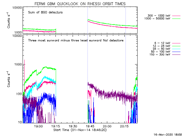
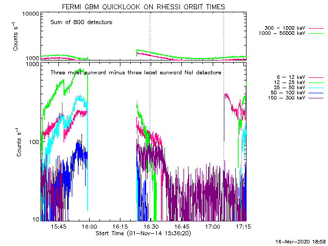
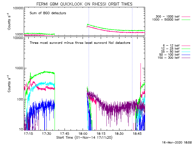
| Nov 1, 2014 | 16:30:10-20:40:09 | 27 ants in config C L: 1-2 GHz/2 MHz, 0.05 s |
Overview dynamic spectrum summary |
VLA_20141101 | B5.1 microflare @19:10 | Yes; 6-12 | Yes; ? | Chen+, ApJ, 2018 |
| C7.2@16:47 | Yes; 6-12 | No | Yu & Chen, ApJ, 2019 | |||||
| C2.3@18.20 | Yes; 6-12 | No | ||||||
| Nov 4, 2014 | 18:06:19-18:43:14 | Config C L/1 MHz, 1 s, S/1 MHz, 1 s, C/1 MHz, 1 s |
-- | 20 dB attn delay calibration | -- | -- | -- | |
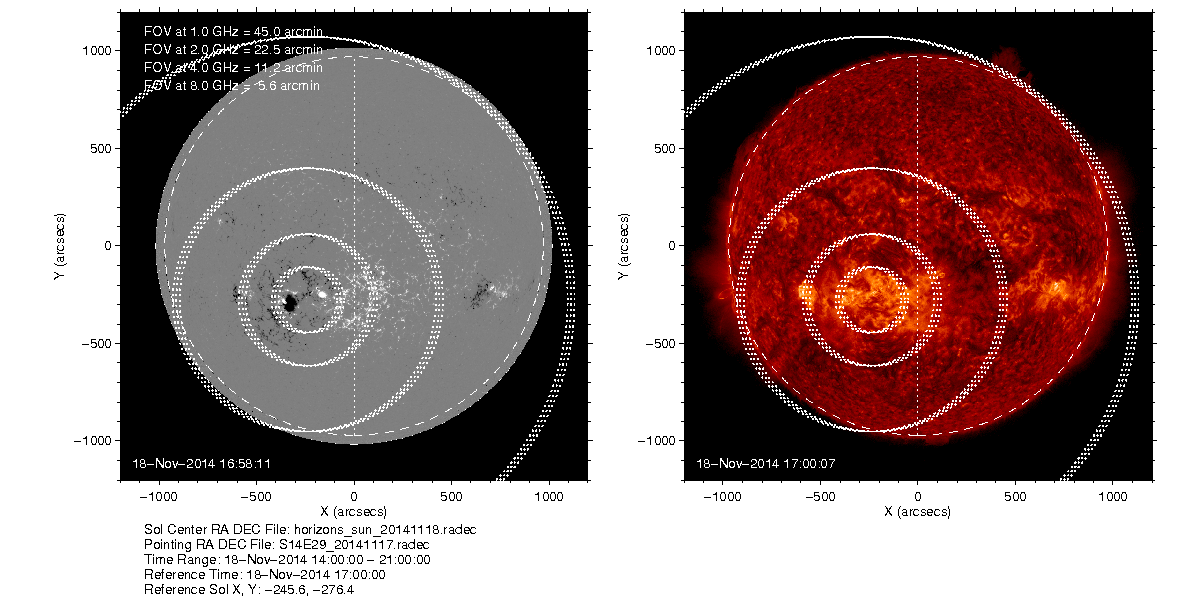
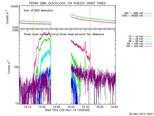
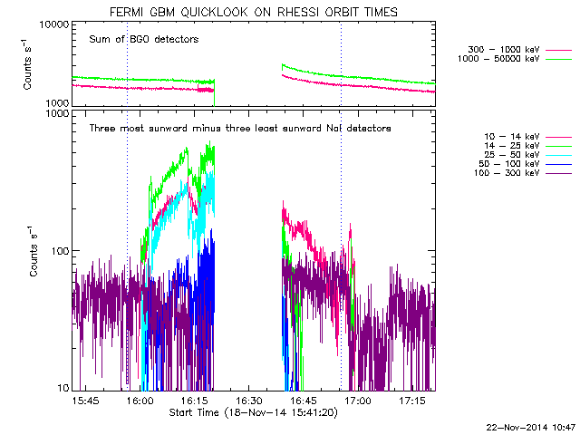
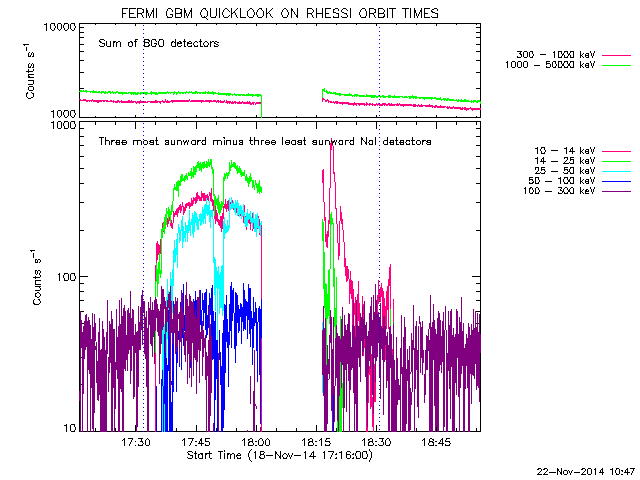
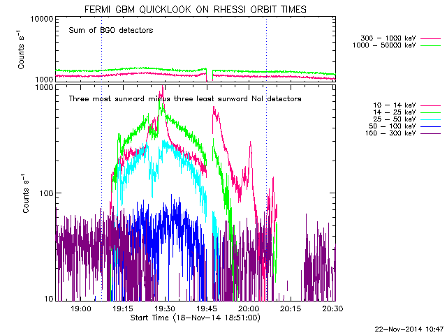
| Nov 18, 2014 | 14:20:46-19:42:51 | Config C L: 1-2 GHz/1 MHz, 1 s; S: 2-4 GHz/1 MHz, 1 s, C: 4-8 GHz/1 MHz, 1 s |
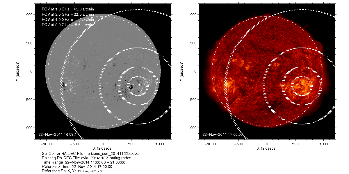
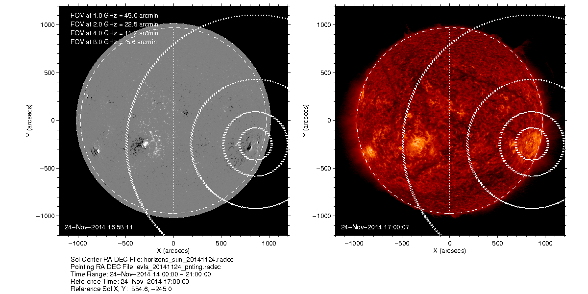
Overview dynamic spectrum FOV |
VLA_20141118 | C2@15:21 | Yes;12-25 | Yes;14-25 | |
| C2@16:45 | No | Yes; 10-14 | ||||||
| C1.6@18:19 | No | Yes; 14-25 | ||||||
| C1.5@19:30 | Yes; 12-25 | Yes; 25-50 | ||||||
| Nov 20, 2014 | 14:12:18-19:41:50 | Config C L: 1-2 GHz/1 MHz, 1 s; S: 2-4 GHz/1 MHz, 1 s, C: 4-8 GHz/1 MHz, 1 s |
Overview dynamic spectrum FOV |
VLA_20141120 | [ C1.2@14:35] | |||
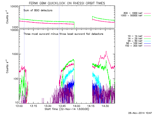
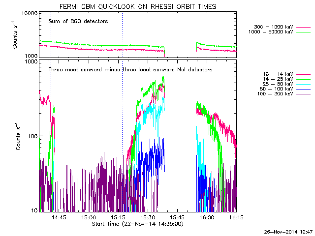
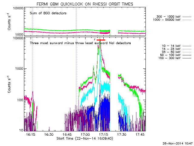
| Nov 22, 2014 | 14:04:32-19:31:35 | Config C L: 1-2 GHz/1 MHz, 1 s; S: 2-4 GHz/1 MHz, 1 s, C: 4-8 GHz/1 MHz, 1 s |
Overview dynamic spectrum FOV |
VLA_20141122 | C2.1@14:36 | Yes;12-25 | No | |
| C2@15:37 | No | No | ||||||
| C2@16:48 | Yes; 6-12 | No | ||||||
| C2@17:13 | No | Yes;50-100 | ||||||
| Nov 24, 2014 | 15:34:00-19:25:47 | Config C L: 1-2 GHz/1 MHz, 1 s; S: 2-4 GHz/1 MHz, 1 s, C: 4-8 GHz/1 MHz, 1 s |
Overview dynamic spectrum FOV |
VLA_20141124 | C1.4@15:56 | Yes; 6-12 | Yes; 10-14 | |
| C2.1@16:20 | Yes;12-25 | No | ||||||
| C2@18:09 | No | No | ||||||
| Dec 8, 2014 | 19:09:27-19:45:36 | Config C L/1 MHz, 1 s, S/1 MHz, 1 s, C/1 MHz, 1 s | -- | 20 dB attn delay calibration | -- | -- | -- | |
| Dec 11, 2014 | 17:48:53-20:50:32 | Config C L: 1-2 GHz/2 MHz, 50 ms |
Overview dynamic spectrum | VLA_20141211 | ||||
| Feb 12, 2016 | 20:50:35-21:05:05 | Config C L: 1-2 GHz/2 MHz, 50 ms |
Overview dynamic spectrum | VLA_20160212 | ||||
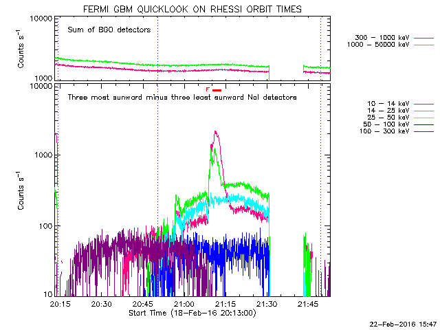
| Feb 18, 2016 | 19:12:29-23:54:05 | 27 ants in Config C 1-2 GHz/2 MHz, 50 ms |
Overview dynamic spectrum summary |
VLA_20160218 | C1.4@20:10 | No | No | |
| C1.8@21:08 | Yes; 12-25 | Yes; 75-100 | Luo+ in prep | |||||
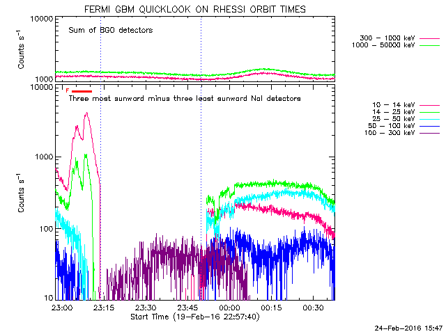
| Feb 19, 2016 | 18:41:49-23:23:25 | 27 ants in Config C 1-2 GHz/2 MHz, 50 ms |
Overview dynamic spectrum summary |
VLA_20160219 | C2.8@23:11 | Yes;6-12 | Yes;14-25 | |
| Feb 23, 2016 | 17:00:06-17:30:07 | Config C L, S, C |
-- | 20 dB attn delay calibration | -- | -- | -- | |
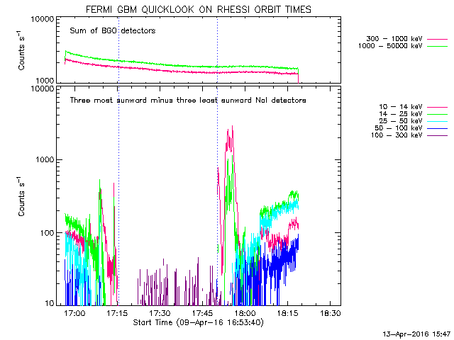
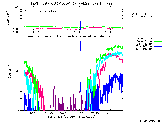
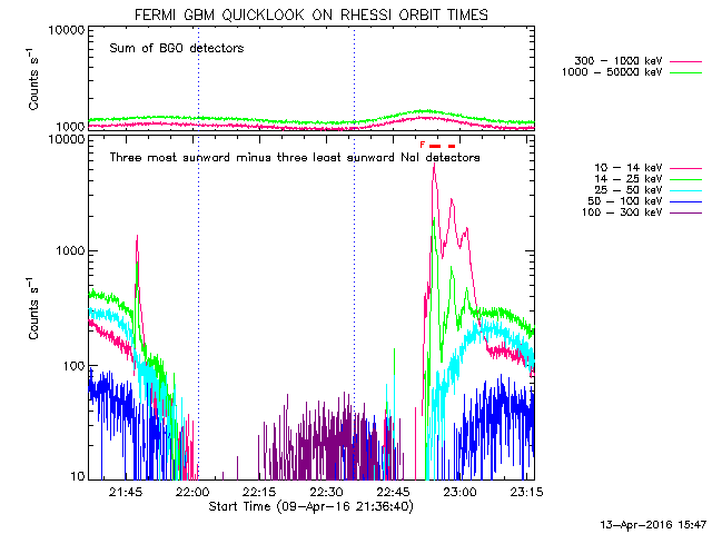
| Apr 09, 2016 | 17:56:59-22:57:52 | 14 ants in Config C 1-2 GHz/2 MHz, 50 ms 13 ants in Config C 1-2 GHz/2 MHz, 50 ms |
Overview dynamic spectrum summary |
VLA_20160409 | C1.7@17:55 | No | Yes;14-25 | |
| C1.5@18:44 | No | Yes; 25-50 | ||||||
| C1.5@20:34 | No | No | ||||||
| C1@20:50 | No | No | ||||||
| C1.4@22:04 | No | No | ||||||
| C1@22:30 | No | No | ||||||
| C1.8@22:54 | No | Yes;14-25 | ||||||
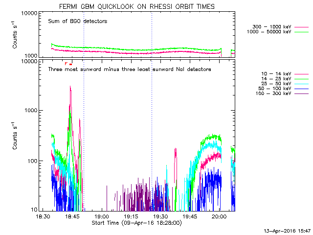
| Apr 10, 2016 | 18:03:25-22:51:40 | Config C L: 1-2 GHz/2 MHz, 50 ms; S: 2-4 GHz/2 MHz, 50 ms |
Overview dynamic spectrum summary |
VLA_20160410 | GOES below C level with microflares; B6.9@21:43 | No | No | |
| Apr 15, 2016 | 17:11:35-22:03:32 | Config C L: 1-2 GHz/2 MHz, 50 ms; S: 2-4 GHz/2 MHz, 50 ms |
Overview dynamic spectrum summary |
VLA_20160415 | GOES below C level with microflares | No | No | |
| Apr 16, 2016 | 17:13:00-22:15:504 | 13 ants in Config C 2-4 GHz/2 MHz, 50 ms |
Overview dynamic spectrum summary |
VLA_20160416 | C1.4@19:14 | No | No | |
| C5.8@19:42 | No | No | ||||||
| Apr 17, 2016 | 17:26:23-22:15:04 | Config C L: 1-2 GHz/2 MHz, 50 ms; S: 2-4 GHz/2 MHz, 50 ms |
Overview dynamic spectrum summary |
VLA_20160417 | C2.4@17:30:00 | No | No | |
| Apr 22, 2016 | 17:12:14-23:04:03 | Config C L: 1-2 GHz/2 MHz, 50 ms |
Overview dynamic spectrum summary |
VLA_20160422 | No | No | ||
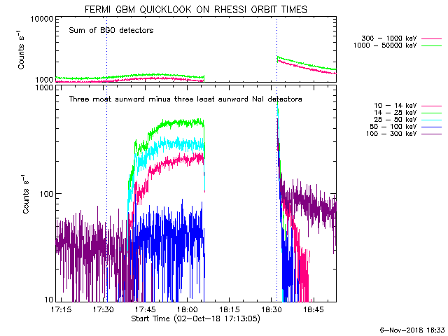
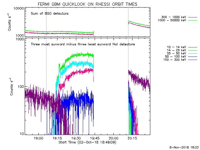
| Oct 02, 2018 | 19:37:23 - 20:07:18 | Config D P: 232-488 MHz/250kHz; 1 s |
First P band test run Dynamic spectrum |
No | No | |||
| Oct 02, 2018 | 17:37:15 - 18:24:30 | Config D L: 1-2 GHz/1MHz; 1 s |
L band test run Dynamic spectrum |
-- | No | Yes | ||
| 18:30:52 - 19:23:25 | L band test run Dynamic spectrum |
-- | No | Yes | ||||
| Oct 3, 2018 | 19:39:55 - 20:04:12 | Config D L: 1-2 GHz/1MHz; 1 s |
L band test run Dynamic spectrum |
No | No |
| ||
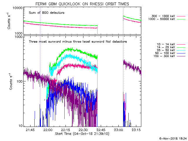
| Oct 4, 2018 | 16:15:06 - 17:51:01 | Config D L: 1-2 GHz/1MHz; 10 ms |
L band test run Dynamic spectrum |
No | No | |||
| Oct 4, 2018 | 17:52:38 - 18:13:12 | Config D P: 232-488 MHz/250kHz; 10 ms |
P band test run Dynamic spectrum |
-- | No | No | ||
| 22:03:53 - 22:33:19 | P band test run Dynamic spectrum |
-- | No | Yes | ||||
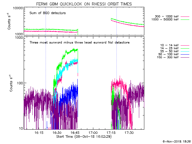
| Oct 08, 2018 | 16:04:32 - 16:24:43 | Config D P: 232-488 MHz/250kHz; 10 ms |
P band test run Dynamic spectrum |
-- | No | Yes | ||
| Oct 08, 2018 | 17:44:43 - 18:08:04 | Config D P: 232-488 MHz/250kHz; L: 1-2 GHz/1MHz; 10 ms |
test run P band Dynamic spectrum L band Dynamic spectrum |
-- | No | No | ||
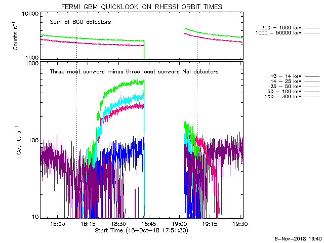
| Oct 15, 2018 | 18:10:05 - 19:18:48 | Config D P: 232-488 MHz/250kHz; L: 1-2 GHz/1MHz; 10 ms |
test run P band Dynamic spectrum L band Dynamic spectrum |
-- | No | Yes | ||
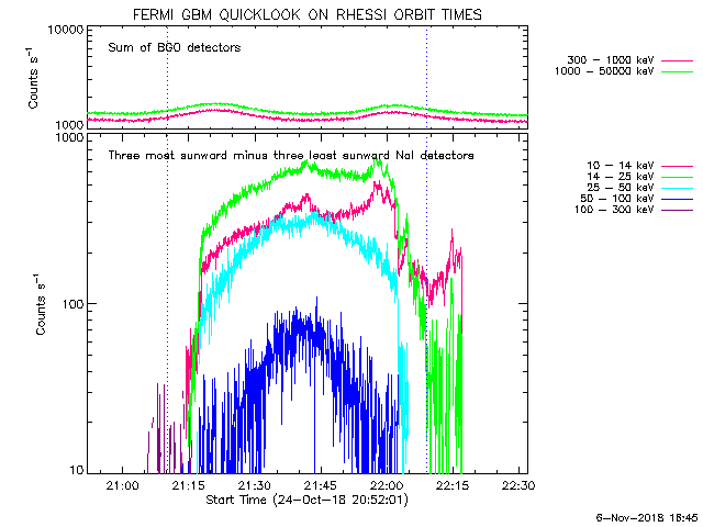
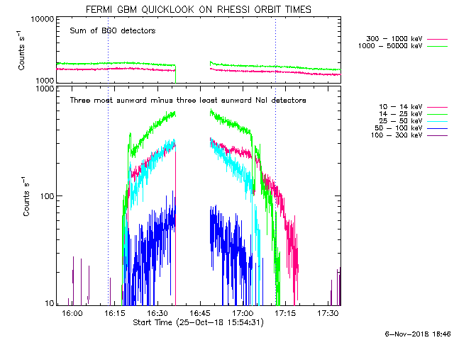
| Oct 24, 2018 | 21:53:11 - 22:00:43 | Config D L: 1-2 GHz/1MHz; 1 s |
Dynamic spectrum | -- | No | Yes | ||
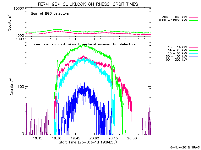
| Oct 25, 2018 | 16:30:00 - 19:40:17 | Config D P: 232-488 MHz/250kHz; L: 1-2 GHz/1MHz; 10 ms |
P band Dynamic spectrum L band Dynamic spectrum |
-- | No | Yes | ||
| 19:44:40 - 21:02:45 | P band Dynamic spectrum L band Dynamic spectrum |
-- | No | Yes | ||||
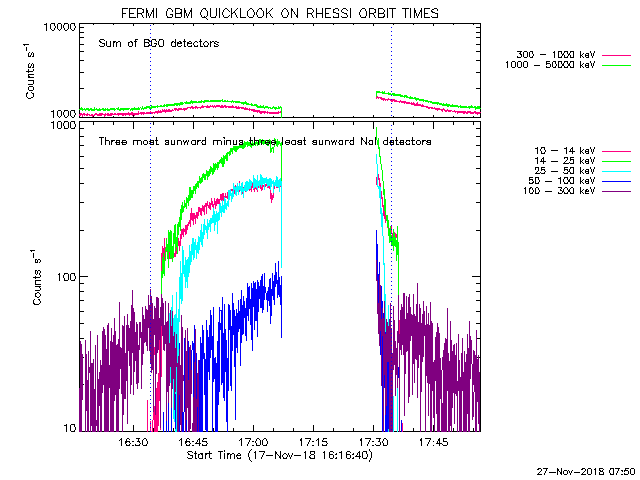
| Nov 18, 2018 | 17:00:00 - 17:45:03 | Config C P: 232-488 MHz/250kHz; L: 1-2 GHz/1MHz; 10 ms |
P band Dynamic spectrum L band Dynamic spectrum |
-- | No | Yes | ||
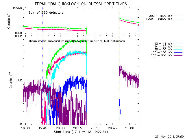
| 18:25:35 - 21:10:03 | P band Dynamic spectrum L band Dynamic spectrum |
successive A-class flares around 18:30 | No | Yes | ||||
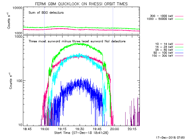
| Dec 7, 2018 | 18:00:00 - 22:10:08 | Config C P: 232-488 MHz/250kHz; L: 1-2 GHz/1MHz; 10 ms |
P band Dynamic spectrum L band Dynamic spectrum |
A8.9 Microflare @19:47 | No | Yes | ||
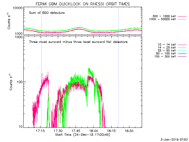
| Dec 24, 2018 | 17:03:41 - 20:14:28 | Config C P: 232-488 MHz/250kHz; L: 1-2 GHz/1MHz; 10 ms |
P band Dynamic spectrum L band Dynamic spectrum |
-- | No | Yes | ||
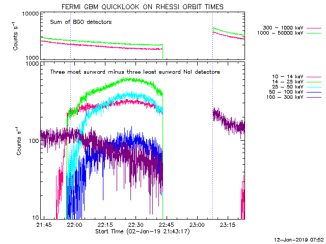
| Jan 2, 2019 | 22:23:38 - 22:28:39 | Config C P: 232-488 MHz/250kHz; L: 1-2 GHz/1MHz; 14 ms |
P band Dynamic spectrum L band Dynamic spectrum |
-- | No | Yes | ||
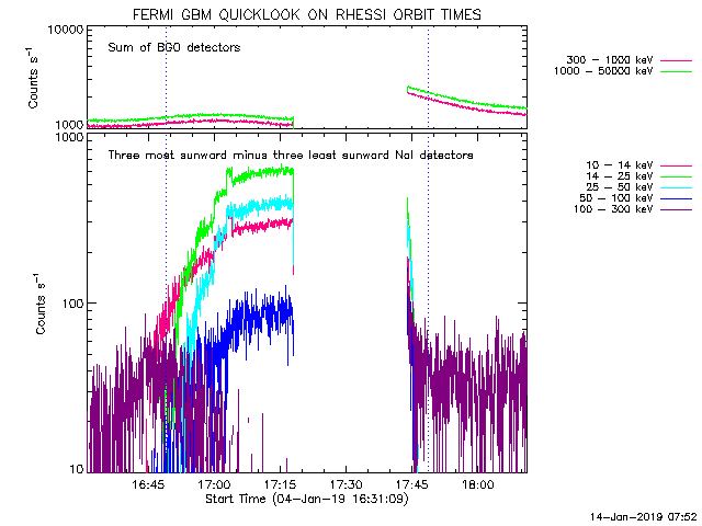
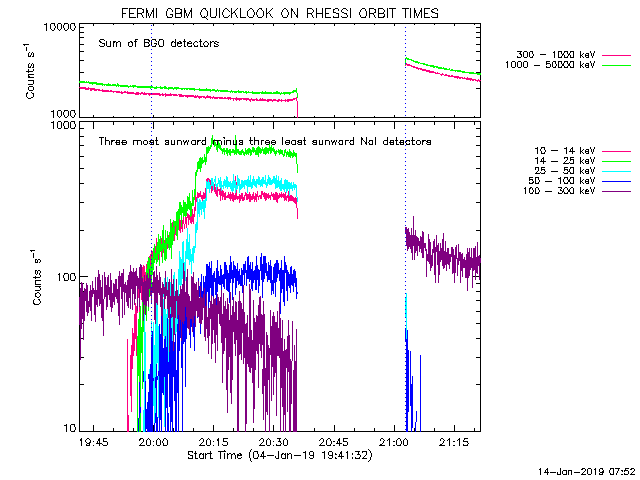
| Jan 4, 2019 | 15:56:55 - 18:11:41 | Config C P: 232-488 MHz/250kHz; L: 1-2 GHz/1MHz; 10 ms |
P band Dynamic spectrum L band Dynamic spectrum |
-- | No | Yes | ||
| 18:33:19 - 21:50:52 | P band Dynamic spectrum L band Dynamic spectrum |
-- | No | Yes | ||||
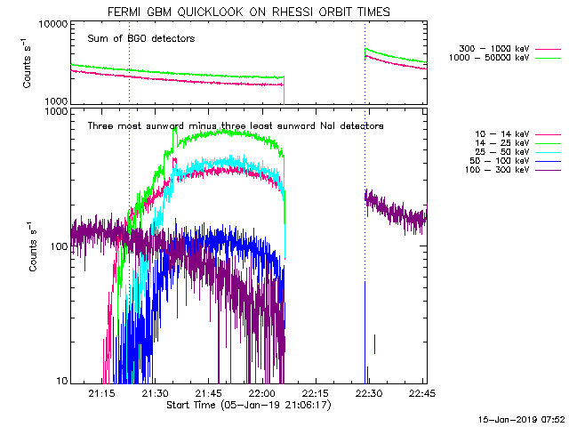
| Jan 5, 2019 | 21:53:24 - 21:58:01 | Config C P: 232-488 MHz/250kHz; L: 1-2 GHz/1MHz; 14 ms |
P band Dynamic spectrum L band Dynamic spectrum |
-- | No | Yes | ||
| 22:29:39 - 22:34:40 | P band Dynamic spectrum L band Dynamic spectrum |
-- | No | Yes | ||||
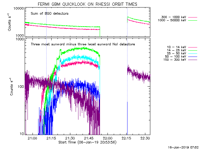
| Jan 6, 2019 | 21:37:03 - 22:16:47 | Config C P: 232-488 MHz/250kHz; L: 1-2 GHz/1MHz; 14 ms |
P band Dynamic spectrum L band Dynamic spectrum |
-- | No | Yes | ||
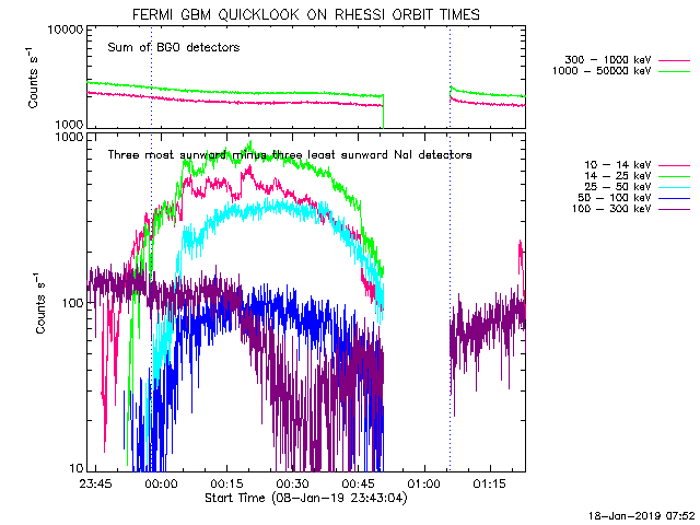
| Jan 7, 2019 | 23:57:55 - 00:02:58 | Config C P: 232-488 MHz/250kHz; 14 ms |
no usable solar scans | -- | No | Yes | ||
| Jan 12, 2019 | 16:06:07 - 17:05:31 | Config C P: 232-488 MHz/250kHz; L: 1-2 GHz/1MHz; 14 ms |
P band Dynamic spectrum L band Dynamic spectrum NuSTAR coordination |
-- | No | Yes | ||
| 17:57:45 - 21:08:15 | P band Dynamic spectrum L band Dynamic spectrum NuSTAR coordination |
-- | No | Yes | ||||
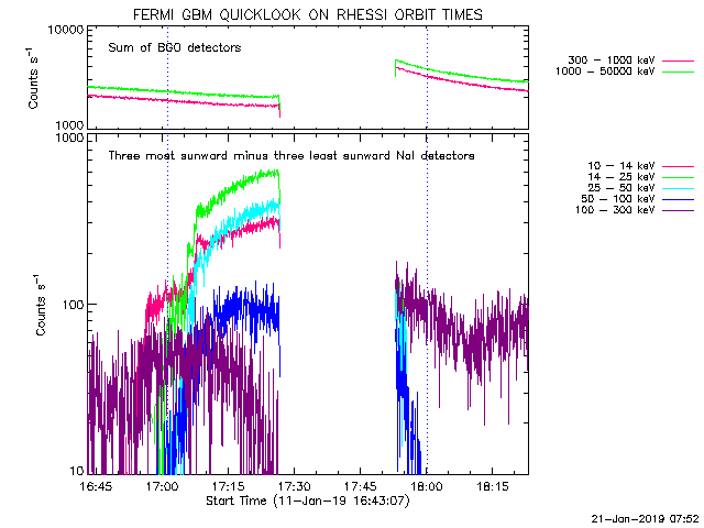
| Jan 17, 2019 | 19:02:28 - 22:57:51 | Config C P: 232-488 MHz/250kHz; 14 ms |
P band Dynamic spectrum | I didn't request this observation | -- | No | Yes | |
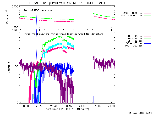
| Jan 25, 2019 | 15:01:59 - 19:20:13 | Config C P: 232-488 MHz/250kHz; L: 1-2 GHz/1MHz; 14 ms |
P band Dynamic spectrum L band Dynamic spectrum |
enormous fine structures in P and L? band spectrum | B2.3 microflare @16:03 | No | Yes | |
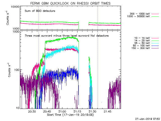
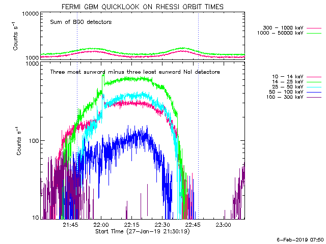
| Jan 27, 2019 | 19:02:28 - 22:57:51 | Config C P: 232-488 MHz/250kHz; L: 1-2 GHz/1MHz; 14 ms |
P band Dynamic spectrum L band Dynamic spectrum |
-- | No | Yes |
Tutorial on Overview Dynamic Spectrum and Imaging
Step 1: Preparation
Get the visibility data
The first step of the data survey is to get the visibility data of the the event you are focusing on. Always the original data should be in the the dictionary '/srg/data/evla', you can find the folders named by the date of the event.
The casa task 'listobs' can help to check the basic information of the data, to get the better understanding of each casa task, you can both type the task name followed with a question mark( for example, 'listobs?') in the server or directly google 'nrao casa listobs'.
For each casa task(take the listobs as a example), you can type 'tget listobs' and then 'inp' to get and change the input parameters then 'go' to run the task.
Task listobs can tell some basic information and task plotants can tell you the configration of the antanas, these are the basic information of your observation data. About the casa task and example of listobs, see the link to CASA guide
The original data may be too large for us to do the survey directly, we can use the task 'split' to split the data.
Using the 2016 Feb 18 event as a example, the original data have 50 millisecond time cadence. To reduce the data size, we average it into 1 second cadence using the "split" command in CASA. The key parameter for doing the averaging is "timebin". Here we set it to "1s", meaning averaging to 1-s cadence. This reduced cadence is very informative for viewing the entire observation. However, if we want to look at structures with full time resolution (e.g., 50 ms), we do not want to do the averaging. But to reduce the data size, we can instead split only a short period (say, 1 minute). In this case, we want to use the "timerange" parameter to select the time range, e.g., "19:10:10~19:11:10" (please follow the output of "help split" for syntax).
taskname           = "split"
vis                =  "/srg/data/evla/20160219/sun_20160219.50ms.ms/"
outputvis          =  "sun-2016021.50ms.ms"
keepmms            =  True
field              =  ""
spw                =  ""
scan               =  ""
antenna            =  ""
correlation        =  ""
timerange          =  "0"
intent             =  ""
array              =  ""
uvrange            =  ""
observation        =  ""
feed               =  ""
datacolumn         =  "data"
keepflags          =  True
width              =  1
timebin            =  "1s"
combine            =  ""
#split(vis="/srg/data/evla/20160219/sun_20160219.50ms.ms/",outputvis="sun-20160219.50ms.ms",keepmms=True,field="",
spw="",scan="",antenna="",correlation="",timerange="",intent="",array="",uvrange="",observation="",feed="",datacolumn="data",keepflags=True,width=1,timebin="1s",combine="")
Other information of the event
Except the vla data itself, we may also need the X-ray data and EUV data to help us. You can see the summary in Prof. Bin's website or go the flare browser and the helioviewer


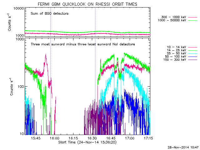
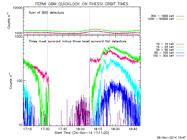
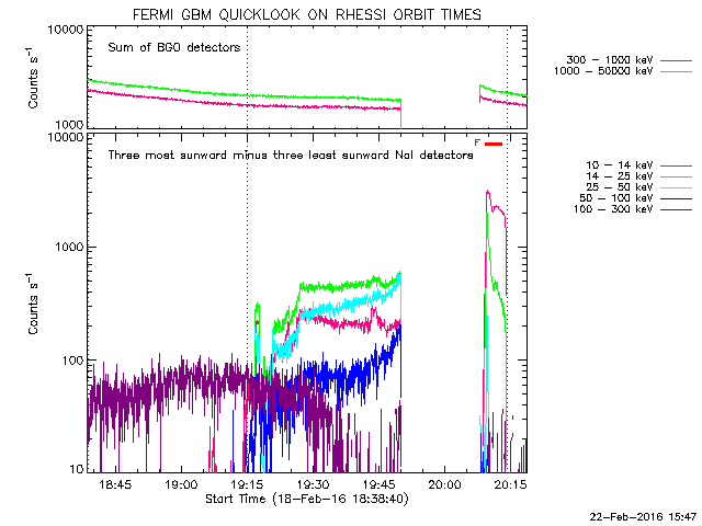
If you are in the server, you can do into idl to get the plot of Goes and RHESSI, which can help us identify the features in the dynamic spectrum.
Type 'goes' or 'hessi' you will see the command window.
Use Goes as a example, when you come into the command window, you can select parameters fot the plotting(mainly the timerange) and after clicking 'plot', you can control the plot in the menus and output the figure or you can directly write the idl savefile(for making the dynamic mivie later) in command window.
Always we need flux and derivate information for analysis.
Step 2: Overview of the Event
Select the appropriate baselines
Usually we use the task 'dspec' to make the dynamic spectrum, use get_dspec to create a npz file, the most important input is timerange and baseline. You can use the casa task 'viewer' to check the visbility data( remember when using the viewer, don not select too long timerange).


When coming into the window of viewer. First in the data manager to select the timerange(no more than 20 minutes) and so on.
Then get into the display panel, set x,y,animation axis as 'time','channel'and'baselines'. Then you can check the display to select propriate baselines. Remember to check every spectral windows and both LCP and RCP.
Check Each baselines and better select both the longer baselines and shorter baselines to make the npz file.
Plot detailed dynamic spectrum
Use plt_dspec to do the plot, after getting the npz file, you can do the plot. Usually we are interested in both LCP and RCP, here set a example.
from suncasa.utils import dspec
msfile = 'sun_20120310A.50ms.ms' # the visbility data
vis = msfile
bl='4&12'
spw='0~7'
specfile = msfile+'.bl4-12.190000-194000.spec.npz'
timeran='17:58:50~17:59:30'
dspec.get_dspec(vis=vis,specfile=specfile,bl=bl,spw=spw,timeran=timeran)
dspec.plt_dspec(specfile=specfile,pol='RR',dmin=1,dmax=12)  #dmin and dmax is used to change color,pol can be selected as 'RR''LL'or'I'

To get the survey of the whole timerange, we need to get a movie, select the movie as True, you can get a folder called 'dspec' which including the figures to make the movie. You can also attach the goes savefile.
After getting the folders, you can use idl to create the movie like this 2012 Mar 10 event or directly use other ways.
Make overview radio/EUV image
Once you find something in the movie, you can back to the origrinal data to see the details, and we can use the calibrated data to make the overview image at that time.
Make radio image (clean)
First step is to make the clean image using CASA task clean, you can also see details od clean in the CASA guide.
Select the appropriate parameters from the dynamic spectrum to do the clean.


Register cleaned CASA image into FITS file
Use the task 'helioimage2fits.imreg' to get the vla_fits file.
from suncasa.utils import helioimage2fits
vis='2110.50ms.cal.ms'
imagfile='2110.image' #clean image
timerange='21:10:31.275~21:10:31.675'
helioimage2fits.imreg(vis=vis,imagefile=imagefile,timerange=timerange)
Plot radio image on AIA
Then add the vla-fits file into the aia map.
from sunpy import map as smap
aiamap=smap.Map('aia_lev1_171a_2012_03_10t17_48_00_34z_image_lev1.fits')
vlafits='1747.fits'
vlamap=smap.Map(vlafits)
vlamap.data = vlamap.data.reshape(vlamap.meta['naxis1'],vlamap.meta['naxis2'])
cmap=smap.CompositeMap(aiamap)
cmap.add_map(vlamap,levels=np.array([0.5,0.7,0.9])*np.nanmax(vlamap.data))
cmap.peek()

You can also zoom in and out to see the details in the image.
Survey overview plot
After you get all the information, you can use the routine 'svplot' to create the overview survey plot.
The required input is the dynamic spectrum file, visbility measurement file, timerange and frequency range. If you have done the clean and get the clean image, you can set the imagefile to your clean image, if you have done the fitsfile, you can set fitsfile to your fitsfile, and if you have downloaded the aiafits, you can set the aiafits to your own aiafits, this steps may save your some time. And you can also change the polarzation by setting pol, the default is 'RRLL'. And you can select the aia wavelength to download by changing aiawave.
To run it in CASA, use command svplot. here is an example import svplotpy(in CASA)
vis='2110.50ms.cal.ms'
spec=2110.spec.npz'
timerange=
spw='2~3‘
svplot.svplot(vis=vis,spec=spec,timerange=timerange,spw=spw)
and you can then get the figures as below.

Make radio movie with svplot
Svplot is also capable to make overview movie from a CASA visibility dataset by setting the keyword mkmovie==True. The following short example shows how to make a movie with svplot from a visibility file.
   from suncasa.utils import svplot as sv
   sv.svplot(vis='IDB20170910T153625-180625.ms.corrected.XXYY.slfcaled',   ## The input ms file.
             timerange='17:00:00~18:06:00'  ## optional, the timerange within which the movie will span over.
             specfile='IDB20170910T153625-180625.ms.corrected.XXYY.slfcaled.dspec.med.npz',   ## optional, will make a new one if not provided
             spw=['1','2','3','4']  ## The spectral window to be imaged. Note: When mkmovie=True,  if spw is a list, images at individual band will be made. If spw is a string, a multi-frequency synthesis image will be made.
             niter=500,
             imsize=[512], ## images size for Clean procedure in unit of pixel
             cell=['2.5arcsec'], ## images resolution for Clean procedure
             xycen=[975, -140], ## The center of images for Clean (Also the center of the image display)
             fov=[512., 512.],  ## field of view of the image display in unit of arcsec
             stokes='XX,YY',
             overwrite=True,  ## If to overwrite the existed fits image files
             mkmovie=True,  ## Set this to True if one want to make a movie
             twidth=12,  ## Number of timestamps to average to form one output image. Say twidth = 12 for an 1 sec integration data, the output time cadence is 12 sec.
             imax=1e7,  ## color scale for the radio image
             imin=0.5e6, ## color scale for the radio image
             dmax=0.5e6, ## color scale for the dynamic spectrum
             plotaia=True, ## optional, set False if you do not want to overlay radio images over AIA EUV images.
             aiadir = './your-aia-data-path', ## if you have the corresponding AIA fits files somewhere locally, provide the folder path. The code will search the following places: 1. the default AIA data path ("/srg/data/sdo/aia/level1/" on baozi); 2. the path provided by keyword "aiadir"; 3. the current directory. If plotaia is True, and there is no aia fits files found at any of the forementioned paths, it will download the specific AIA fits data to the current directory.
             aiawave=171,  ## optional, AIA passband.
             plt_composite=True,  ## optional, set True if you want to plot radio image contours from all specified spectral windows in one images.
             ncpu=10)
The resulting images will be saved to "qlookimgs" folder under the current directory.
Example 1: Radio image movie with no AIA files provided.
Example 2: Radio image movie with AIA images in the background.
Example 3: Radio images from different spectral windows combined in one plot.