Antenna Position

Fundamentals

A synthesis imaging radio instrument consists of a number of radio elements (radio dishes, dipoles, or other collectors of radio emission), which represent measurement points in u,v,w space. We need to describe how to convert an array of dishes on the ground to a set of points in u,v,w space.

E, N, U coordinates to x, y, z

The first step is to determine a consistent coordinate system. Antennas are typically measured in units such as meters along the ground. We will use a right-handed coordinate system of East, North, and Up (E, N, U). These coordinates are relative to the local horizon, however, and will change depending on where we are on the spherical Earth. It is convenient in astronomy to use a coordinate system aligned with the Earth's rotational axis, for which we will use coordinates (x, y, z) as shown in Figure 1. Conversion from (E, N, U) to (x, y, z) is done via a simple rotation matrix:

Fig. 1: The relationship between E, N, U coordinates and x, y, z coordinates, for a latitude $\lambda$. The direction of z is parallel to the direction to the celestial pole. The directions y and E are the same direction.

${\begin{bmatrix}x\\y\\z\\\end{bmatrix}}={\begin{bmatrix}0&-\sin \lambda &\cos \lambda \\1&0&0\\0&\cos \lambda &\sin \lambda \\\end{bmatrix}}{\begin{bmatrix}E\\N\\U\\\end{bmatrix}}$

which yields the relations:

${\begin{aligned}x&=-N\sin \lambda +U\cos \lambda \\y&=E\\z&=N\cos \lambda +U\sin \lambda \end{aligned}}$

Baselines and Spatial Frequencies

Note that the baselines are differences of coordinates, i.e. for the baseline between two antennas we have a vector:

Fig. 2: Geometry of an interferometer baseline where a delay $\tau$ is inserted in one antenna, in order to steer the phase center to a direction $\theta _{o}$ from the vertical $\lambda$.

${\vec {B}}=(B_{x},B_{y},B_{z})=(x_{2}-x_{1},y_{2}-y_{1},z_{2}-z_{1})$

This vector difference in positions can point in any direction in space, but the part of the baseline that matters in calculating u,v,w is the component perpendicular to the direction $\theta _{o}$ (the phase center direction), which we called $B_{proj}$ in Figure 2. Let us express the phase center direction as a unit vector ${\vec {s_{o}}}$ $=(h_{o},\delta _{o})$, where $h_{o}$ is the hour angle (relative to the local meridian) and $\delta _{o}$ is the declination (relative to the celestial equator). Then $B_{proj}={\vec {B}}\cdot {\vec {s_{o}}}=B\cos \theta _{o}$.

Recall that the spatial frequencies u,v,w are just the distances expressed in wavelength units, so we can get the u,v,w coordinates from the baseline length expressed in wavelength units from the following coordinate transformation (see Thompson 1999 for details):

${\begin{bmatrix}u\\v\\w\\\end{bmatrix}}={\vec {B_{\lambda }}}\cdot {\vec {s_{o}}}=(1/\lambda ){\begin{bmatrix}\sin h_{o}&\cos h_{o}&0\\-\sin \delta _{o}\cos h_{o}&\sin \delta _{o}\sin h_{o}&\cos \delta _{o}\\\cos \delta _{o}\cos h_{o}&-\cos \delta _{o}\sin h_{o}&\sin \delta _{o}\\\end{bmatrix}}{\begin{bmatrix}B_{x}\\B_{y}\\B_{z}\end{bmatrix}}$ $(1)$

How baseline errors can contribute to the error in phase

The geometric phase difference at the phase center ($w$ term in (1)) is:

$\phi _{g}=2\pi \tau _{g}\nu =(2\pi /\lambda )[B_{x}\cos \delta _{o}\cos h_{o}-B_{y}\cos \delta _{o}\sin h_{o}+B_{z}\sin \delta _{o}]$

where $\tau _{g}={\vec {B}}\cdot {\vec {s}}/c$, geometric delay. We can see what can affect the geometric phase by taking the differential of this expression:

${\begin{aligned}d\phi _{g}=2\pi \nu d\tau _{g}=(2\pi /\lambda )[&dB_{x}\cos \delta _{o}\cos h_{o}-dB_{y}\cos \delta _{o}\sin h_{o}+dB_{z}\sin \delta _{o}\\+\ &d\alpha _{o}\cos \delta _{o}(B_{x}\sin h_{o}+B_{y}\cos h_{o})\\+\ &d\delta _{o}(-B_{x}\cos h_{o}\sin \delta _{o}+B_{y}\sin h_{o}\sin \delta _{o}+B_{z}\cos \delta _{o})]\end{aligned}}$$(2)$

where we have used the relation between right ascension and hour angle: $h_{o}=LST-\alpha _{o}$, so $dh_{o}=-d\alpha _{o}$. Equation (2) shows how baseline errors $(dB_{x},dB_{y},dB_{z})$ and source position errors ($\alpha _{o}$, $\delta _{o}$) will affect the error in group delay $d\tau _{g}$ (or yield an error in phase $d\phi _{g}$). Note that a clock error is equivalent to a source position error $d\alpha _{o}$.

If we have a source whose position is known, we can use Equation (2) to find the location of the antennas (this is called baseline determination). The error in antenna position is largely independent of the baseline lengths. For example, say that we can measure $d\phi _{g}$ to within 1 degree at 5 GHz ($\lambda$ = 6 cm). Then we can measure $dB_{x}$, $dB_{y}$ and $dB_{z}$ to a precision of order (1 / 360) 6 cm ~ 1 / 60 cm even though $B=(B_{x}^{2}+B_{y}^{2}+B_{z}^{2})^{1/2}$ = 5000 km or more (VLBI).

The time of day and location of the antennas must be known to relatively high accuracy -- needed for determining the geometric delay. A clock error of 1 s, or a baseline error of a few cm, will cause a serious phase shift of the source over, say, 10 minutes. At OVRO, using a GPS clock and measuring baselines with cosmic source calibration, we get a time accuracy of << 1 ms, and baseline errors of about 3 mm. Therefore, these effects are not serious over a short time interval, but may still be problematic over 8 hours. This is one reason that we do phase calibration observations every ~ 2 hours.

EOVSA Antenna Position Calibration

The positions of EOVSA antennas are determined using observations by the 27-m (Ant 14) low-frequency receiver (S and C band) of celestial radio sources during several observation runs in fall 2016. This document describes the procedure followed and the final? calibrated antenna positions.

For calibrator sources with locations with sufficient accuracy (we use caibrators from the VLA Calibrator Manual), and a good time-keeping accuracy at EOVSA (what is our time-keeping accuracy? --Bchen 19 November 2016) , $d\alpha _{o}$ and $d\delta _{o}$ in Eq. 2 can be neglected. Hence Eq. 2 can be simplified to:

$\phi _{g}=\phi _{o}+(2\pi /\lambda )(dB_{x}\cos \delta \cos h-dB_{y}\cos \delta \sin h+dB_{z}\sin \delta )$, (3)

where $\phi _{o}$ is the intrinsic instrumental phase at the given baseline.

We use a two-step calibration to solve for the EOVSA baseline error as following:

1. Determine baseline errors in X and Y

Observing one strong and point-like calibrator for a sufficiently long time (at least several hours). Note it is important to observe for a long time in order to have sufficient variation of the phase vs. hour angle curve as determined by sin(h) and cos(h). We use a function of the following form to fit the observed phases at a baseline involving antenna i and j:

$\phi _{ij}=(2\pi /\lambda )(c_{0}+c_{1}\cos h+c_{2}\sin h)$

where

${\begin{aligned}c_{0}&=\phi _{oij}/(2\pi /\lambda )+\sin \delta (dB_{zi}-dB_{zj})\\c_{1}&=\cos \delta (dB_{xi}-dB_{xj})\\c_{2}&=-\cos \delta (dB_{yi}-dB_{yj})\end{aligned}}$ (4)

In a usual case, visibilities are measured at many baselines (e.g., for N antennas one would normally have N(N-1)/2 unique baselines). In that case, one can solve for the antenna-based phase $\phi _{i}$ as a function of hour angle for each antenna i. The resulted fit parameters c₁ and c₂ then only involve the absolute position error dB_i for antenna i. For EOVSA, we only have one 27-m antenna in the array, so we have to use the 13 baseline-based phases $\phi _{i-14}$ to solve for $dB_{(x,y,z)i}-dB_{(x,y,z)14}$. For simplification, I will omit the subscripts (i-14) In the following discussions.

For each antenna i-14 baseline pair, we have two unique polarization measurements. To take advantage of both polarization measurements, we fit the following equations separately:

${\begin{aligned}\phi _{XX}+\phi _{YY}&=(2\pi /\lambda )(c_{0XX}+c_{0YY}+2c_{1}\cos h+2c_{2}\sin h)\\\phi _{XX}-\phi _{YY}&=(2\pi /\lambda )(c_{0XX}-c_{0YY})\end{aligned}}$ (5)

and obtain the four parameters $c_{0XX}$, $c_{0YY}$, $c_{1}$, and $c_{2}$. The baseline error for antenna i (relative to antenna 14) is then:

${\begin{aligned}dB_{x}&={\frac {c_{1}}{\cos \delta }}\\dB_{y}&=-{\frac {c_{2}}{\cos \delta }}\\\end{aligned}}$ (6)

An example is given in Fig. 3 based on a 5.5-hr observation on 3C84 made on 2016 Sep 7 using EOVSA band 5 only (7 usable science channels).

Fig. 3: Phase vs. hour angle for Antennas 9, 10, 11, 13 w.r.t. Antenna 14 at both XX and YY polarizations. This is based on a ~5.5 hour observation of 3C84 on 2016 Sep 7. Circular symbols are measured phases and curves are the corresponding sinusoidal curves. Different colors represent measurements/fits at different frequency channels.

After $dB_{x},dB_{y}$ are determined, they can be applied to the visibility date to correct for the sinusoidal variation of the phase vs. hour angle. I use CASA's task "gencal" to generate the calibration table for antenna position correction (use mode="antpos"). However, the task requires corrections of the antenna positions in the ITRF (International Terrestrial Reference Frame) coordinate system (see gencal help page for details). The X-axis of this system points to prime meridian, i.e., the big circle along zero longitude, while the X-axis of our local Cartesian x, y, z system points to the local central meridian. Therefore we have to rotate the derived $dB_{x},dB_{y}$ by EOVSA's longitude (118.287° west, or -118.287°) to get the new $dB_{x}',dB_{y}'$ in the ITRF system:

${\begin{aligned}dB_{x'}&=dB_{x}\cos(l)-dB_{y}\sin(l)\\dB_{y'}&=dB_{x}\sin(l)+dB_{y}\cos(l)\\\end{aligned}}$ (7)

Each antenna should have three inputs in "parameter": $dB_{x}',dB_{y}',dB_{z}'$. For now we set $dB_{z}'$ to be 0, which will be determined in the next step. An example of generating a calibration table and apply the corrections for the positions of antenna IDs 8 and 9 (that is, Ant 9 and 10):

gencal(vis=your_ms_visibility,caltable='caltb.antpos',caltype='antpos',
            antenna='8, 9', parameter=[dBx'_9, dBy'_9, 0, dBx'_10, dBy'_10, 0])
applycal(vis=your_ms_visibility,gaintable='caltb.antpos')

The results after applying the B_x and B_y correction are shown in Fig. 4:

Fig. 4: Corrected phase vs. hour angle for Antennas 9, 10, 11, 13 w.r.t. Antenna 14 at both XX and YY polarizations. This is based on a ~5.5 hour observation of 3C84 on 2016 Sep 7. Different colors represent measurements/fits at different frequency channels.

Each frequency channel has an independent measurement of the correlated phases (note the wavelength λ in Eq. 3 is different). But they should return the same answer of dB_x and dB_y. Previously I selected 6 channels in Band 5 and fit them independently, and took the average of the resulted dB_x and dB_y to be the answer. This worked pretty well for the 2016 Sep 7 observation on 3C84, which is a very strong calibrator source (23 Jy in C band) and we observed band 5 in a sit-and-stare mode, hence the signal-to-noise was excellent at all channels (results are shown in Figs. 3 and 4). However, for calibrators that are not so strong and/or the array in a fast-frequency-tuning mode, the signal-to-noise is not so good. Fitting all channels independently would result in different answers, especially for those with small baseline errors. An example is shown in Fig. 5 for an observation on 2016 Oct 9 on 2253+161 using the fast frequency-sweeping mode. It is desired to take data from all channels and fit for the same c₁ and c₂ (which are determined by dB_x and dB_y respectively), but different c₀ parameter in Eq. 4 (because different channels have different phase offsets). I have implemented such a technique using SciPy's "leastsq" function. I applied this method to an observation of 2136+006 (9.9 Jy at C band) and 2253+161 (10 Jy at C band) on 2016 Sep 7 under the fast frequency-sweeping mode of the 27-m low-frequency receiver. The results are shown in Fig. 6.

• 

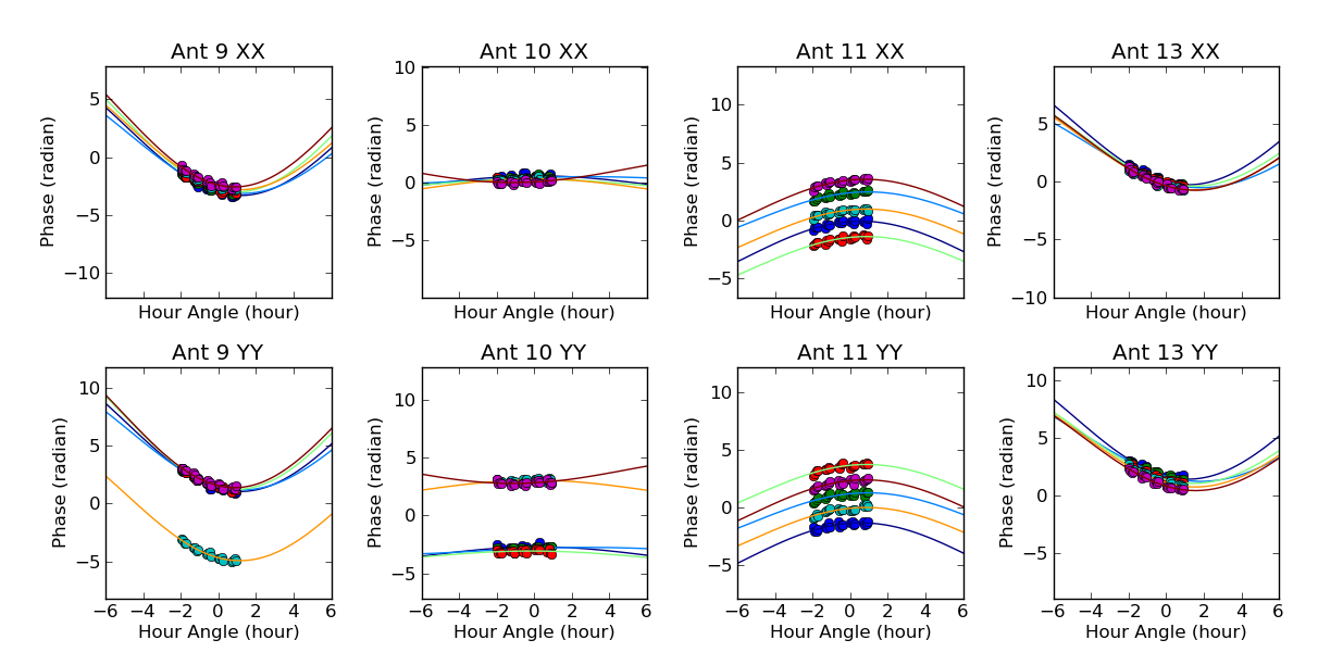
  Phase vs. hour angle for Antennas 9, 10, 11, 13 w.r.t. Antenna 14 at both XX and YY polarizations. Fits are done on each channel independently.

• 

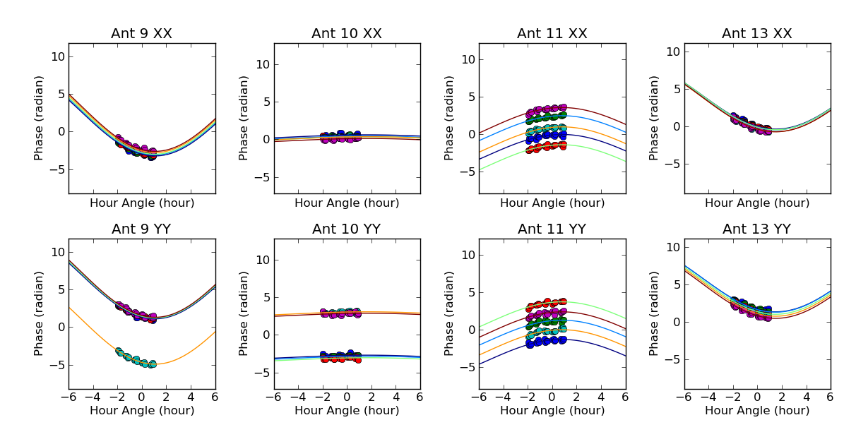
  Phase vs. hour angle for Antennas 9, 10, 11, 13 w.r.t. Antenna 14 at both XX and YY polarizations. Fits are done on all channels simultaneously.

Table 1: Calculated Baseline Corrections in X and Y
Antenna	dBx (m)			dBy (m)
	3C84	2136+006	2153+161	3C84	2136+006	2153+161
	2016/09/07	2016/10/09	2016/10/09	2016/09/07	2016/10/09	2016/10/09
eo09	-0.075	-0.061	-0.064	0.018	0.019	0.018
eo10	-0/006	0.003	0.003	0.004	0.001	-0.001
eo11	0.028	--	0.030	-0.011	--	-0.006
eo13	-0.029	-0.049	-0.047	0.013	0.024	0.020

2. Determine baseline errors in Z

Once the B_x and B_y coordinates have been determined, there should not be significant phase change as a function of time. The remaining error is in B_z, which results in different phases for sources at different declinations. From Eq. 3 we now have:

$\phi _{g}=\phi _{o}+(2\pi /\lambda )dB_{z}\sin \delta$ (8)

We can now observe several calibrator sources at different declinations δ, and fit a function to the observed phases as below:

$\phi =(2\pi /\lambda )(c_{3}+c_{4}\sin \delta ),$ (9)

where $c_{4}=dB_{z}$ is the resulted baseline error in Z. We had an observation on 2016 Oct 9 on two calibrator sources at different declinations (2136+006 and 2153+161), which is used to determine a rough value of dB_z. However, it is desired to make an observation on many more sources to fit the sinusoidal curve to improve the accuracy. Our calibrator survey performed on 2016 Oct 14 would be a good database to do this. We need to firstly apply the B_x and B_y corrections to the visibility data, and then fit the phases at different declinations.

Source Coordinates

The source catalog uses the framework provided by the aipy (astronomical imaging in python) package, which in turn is based on the pyephem package. Source coordinates in pyephem are available in three systems:

• a_ra, a_dec — Astrometric Geocentric Position in J2000 (or ICRF) coordinates (or another epoch if specified)
• g_ra, g_dec — Apparent Geocentric Position for the epoch-of-date
• ra, dec — Apparent Topocentric Position for the epoch-of-date

Unfortunately, CASA wants the source Astrometric Topocentric Position in J2000 coordinates, which is none of the above. However, it is sufficient to calculate the difference between apparent topocentric and apparent geocentric coordinates, and then add it to the astrometric geocentric coordinates, i.e.

• ra_j2000 = (src.ra - src.g_ra) + src.a_ra
• dec_j2000 = (src.dec - src.g_dec) + src.a_dec

Of course, for very distant sources this correction is unnecessary.

For moving sources, such as the Sun, the RA and Dec coordinates are continually changing. For that reason, it is necessary to know the time for which the coordinates are valid. EOVSA Miriad files use the start time of the scan.