GSFIT Help

GSFIT Installation

Launching the GSFIT GUI Application

The GSFIT interactive GUI application may be launched as follows

IDL> gsfit [,nthreads]

where nthreads is an optional argument that indicates the number of parallel asynchronous threads to be used when performing the fit tasks. By default, GSFIT launches with only one thread, but the user may interactively add or delete threads as needed at the run-time up to the number of CPUs available on the system. After some delay while the interface loads, the GUI below should appear.

GSFIT GUI appearance on Windows OS
GSFIT GUI appearance on Linux/Mac OS

The GSFIT GUI is organized in three main sections:

GSFIT Top Main Menu Toolbar, which may be used to perform most of the actions.
GSFIT Left Panel, which displays a microwave map corresponding to the observing frequency and time instance selected via two horizontal scroll bars.
GSFIT Middle Panel, which displays the microwave spectrum corresponding to the selected pixel in the right panel map.
GSFIT Right Panel, which consists of three main elements:
- GSFIT List Scrollbar, which allows the user to locate spatially and temporarily the fit already performed and inspect the fit results
- GSFIT Settings page, which allows the user to setup a series of the spectral fit options and perform some actions via a local Toolbar menu.
- GSFIT Task Queue page, which displays a list of completed, active, and pending fitting tasks.

GSFIT Top Main Menu Toolbar

This toolbar contains a series of action buttons described below.

Upload EOVSA Map Cube

EOVSA map cubes are IDL sav files containg a [ntimes x nfrequencies] brightness temperature (Tb) map structure. Follow this link to learn how such EOVSA map cubes are produced. When uploaded, GSFIT converts these Tb maps to Solar Flux (total intensity or circular polarization) maps. A demo EOVSA map cube is distributed with the GSFI package, being located in the "..//gsfit/demo" directory. To learn more about the structure of the EOMAPS variable saved in this demo file, which is the structure expected by GSFIT in order to recognize and accept such variable as a valid data input, please visit GSFIT Data Format.

Select Color Table

Use this button to select a color table for displaying the microwave maps and spectra. GSFIT uses as default the IDL color table #39 (Rainbow+White)

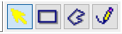Select Mouse Mode

Use this set of mutual exclusive radio buttons to switch between four modes of mouse tool operation.

FOV/Pixel Selection Mode: Use this mouse mode to zoom in and out the field of view (FOV) of the microwave maps displayed on the GSFIT Left Panel, or to select the pixel for which the microwave spectrum is displayed in theGSFIT Middle Panel.
- To zoom in, press, hold, move, and release the left mouse button to select the desired rectangular FOV (rubber-band selection process). To revert to the full FOV, use a single left-button click.
- Use the right button to select a map pixel on the GSFIT Left Panel. The currently selected pixel is indicated by a set of horizontal and vertical dotted lines. Alternatively, the pixel may be selected using the Cursor X and Cursor Y numerical controls located below the map plot area.
Rectangular ROI Selection Mode: Use this mouse mode to define a rectangular region of interest (ROI) through a left button rubber-band selection process. The selected ROI is preserved and displayed as long it is not replaced by another ROI selection, or deleted by a single left button click.
Polygonal ROI Selection Mode: Use this mouse mode to define the vertices of polygonal ROI through a series of sequential left button clicks. To finalize the process, use a right button click to define the last vertex, which will be automatically connected with the first one. The selected ROI is preserved and displayed as long it is not replaced by another ROI selection, or deleted by a single left button click.
Free-hand ROI Selection Mode: Use this mouse mode to define an arbitrarily shaped ROI contour through a continues movement of the mouse cursor while the left button is pressed. To finalize the process, release the left button to define the last vertex of the countour, which will be automatically connected with the first one. The selected ROI is preserved and displayed as long it is not replaced by another ROI selection, or deleted by a single left button click.

Save ROI

Use this button to save to an IDL file the current ROI selection as a set of two arrays, xroi and yroi, containing its vertex heliocentric coordinates.

Restore ROI

Use this button to import from an IDL file a set of xroi and yroi ROI vertex coordinates previously saved by GSFIT, or generated by alternative means.

Select Fit Frequency Range

Use this set off drop lists controls to select the frequency range to be used for spectral fitting. By default, the full frequency range is selected when a map data cube is uploaded, but the user may choose to restrict this default frequency range for various reasons, such as data quality, or apparent source nonuniformity.

Fit Selected Pixel

Use this button to fit the microwave spectrum displayed on the GSFIT Middle Panel using the selected fit frequency range and the settings displayed on the GSFIT Settings panel.

Fit Range

Use this button to perform one or more of the following actions:

Define a rectangular ROI starting at the current cursor position, if no ROI has been previously defined
Select a time range and time resolution for producing a sequence of fits for each ROI pixel
Ignore the current ROI and Time Range selections and choose instead to fit the entire map cube
Use or change the current FIT Frequency Range selection
Enqueue and start processing the fitting of all ROI pixels over the user-defined time interval (default)
Enqueue and Wait for future processing of the fit task of all ROI pixels over the user-defined time interval
Generate and save the fit task for future batch processing by the GSFIT Command Prompt (GSFITCP) application.

Depending on whether or not a ROI is already defined, the user is exposed to a different dialog box to define a fitting task.

Fit Task Dialog Box if no ROI has been already defined
Fit Task Dialog Box if a ROI has been already defined

To enqueue the fit tasks for immediate or future processing by GSFIT, the following rules are followed:

All ROI spectra from a given time frame are processed simultaneously by being as evenly as possible assigned to all active asynchronous parallel threads

The individual time frames are enqueued and processed sequentially

An example about how the tasks are scheduled is provided in the GSFIT Task Queue section.

NOTE: If a fit task is saved for future batch processing, the scheduling is performed at runtime by the GSFIT Command Prompt (GSFITCP) application using the number of active parallel threads available to it.

Abort/Delete Tasks

Use this button to select one of the options from the Delete Options dialog box.

Process Pending Tasks

Use this button to start processing all pending tasks in the GSFIT Queue

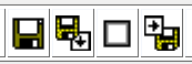Fit List Toolbar Actions

This collection of toolbar buttons provide the following options:

Save Fit List: use this option to save the list of fit solutions, if any, to an IDL *.sav file
Restore Fit List: use this option to restore a previously saved list of fit solutions. Note that this action is successful only if an input data file is already open and the stored fit list is compatible with it!
Send Fit List to GSFITVIEW: use this button to send the current fit list to the GSFITVIEW GUI Application for visualization and inspection.
Export Fit List as an IDL Parameter Map Structure: use this button to convert the current fit list to an IDL parameter map structure that can be open by the GSFITVIEW GUI Application for visualization and inspection.

To learn more about the fit list or parameter maps data structures, and how they may be restored outside the GSFIT application for command line or programmatic manipulation, please visit GSFIT Data Format.

GSFIT Help

Use this button to automatically open this webpage (Windows OS only) or to display the url of this page (Linux/Mac OS).

Number of parallel threads

Use this button to increase or decrease at runtime the number of asynchronous parallel thread used by GSFIT. This input is bounded between 1 and the number of available CPUs. To avoid unnecessary use of CPU resources, GSFIT always launch with only one parallel asynchronous thread.

GSFIT Left Panel

This GSFIT GUI section contains the following elements:

Frequency Selector Scrollbar, which selects the EOVSA map to be displayed. The currently selected pixel is marked by the two vertical and horizontal dotted lines, and the ROI contour is also shown by a continous line, if any defined (see here how).
Map Display Area, where the map selected using the frequency and time scrollbars is displayed
Manual Cursor X and Cursor Y Controls, which provides an alternative to the mouse right-button click for selecting a particular map pixel
Plot character size control, which allows adjustments of the plot character size used in both right and middle panel display areas
Integrated Flux Threshold Checkmark, which, when selected, displays only the map pixels that survive the Integrated Flux Threshold set by the user in the GSFIT Settings page

a: Selected EOVSA map displayed with no Integrated Flux Threshold applied and a free-hand ROI contour.
b: Selected EOVSA map displayed with 1 sfu Integrated Flux Threshold applied and no ROI defined.

GSFIT Middle Panel

This GSFIT GUI section contains the following elements:

Time Selector Scrollbar, which selects the instances corresponding to the map displayed in the left panel and the spectrum displayed in the spectral plot area
Spectral Plot Area, which displays the spatially-resolved microwave spectrum corresponding to the pixel selected in the left panel. The frequency selected on the left panel is shown in the spectral plot by a vertical dashed line. The frequency-dependent errors bars displayed in this plot are computing $err(freq)=rms(freq)+rmsweight\times \max(rms(freq))/freq$ , where rms and freq are provided by the input map structure, and rmsweight is a weighing factor that accounts for the frequency-dependent map resolution. The default rmsweight factor may be adjusted by the user in the GSFIT Settings page.

a: Spectrum corresponding to the selected time frame and selected pixel on the left panel
b: Spectral plot with overlaid Fast Code guess parameters solution (cyan)
c: Spectral plot with overlaid GSFIT (green) and Fast Code (cyan) guess parameters solutions
d: Spectral plot with overlaid GSFIT (green) and Fast Code (cyan) solutions

GSFIT Right Panel

The GSFIT Right Panel consists of three main components:

GSFIT List Scrollbar
GSFIT Settings
GSFIT Task Queue

These components are described below.

GSFIT Right Panel with the GSFIT Settings page displayed

GSFIT List Scrollbar

This scrollbar may be used to navigate through the list of already computed fit solutions, if any. The scrollbar displays the selected solution index and the total number of computed solutions. These fit solutions are indexed in the order in which they are processed by the Task Queue, thus they may not be necessarily clustered in space or time.

Upon selection of a particular fit index the following actions are automatically performed:

The time frame corresponding to the fit is selected and displayed on the Time Scrollbar
The corresponding data map at the frequency currently selected by the Frequency Scrollbar is displayed in the Left Panel
The Right Panel cursor is moved to the corresponding pixel position, which is also displayed by the Cursor X and Cursor Y controls located below the Right Panel plot area
The microwave spectrum corresponding to the selected pixel position and time frame is displayed in the Middle Panel and the fit solution is overlaid.

Upon selection of a particular pixel and time frame by use of the mouse, numerical cursors, or the time scrollbar that matches an already computed fit solution, the fit solution is overlaid on the Middle Panel spectral plot, and the GSFIT List Scrollbar is moved to the matched fit index.

GSFIT Settings

GSFIT Input Parameter Fields

This page exposes to the users a series of editable input fields, as well as a few non-editable fields that are automatically populated by GSFIT based on actions taken by the user in other sections of the GUI. All these fields are described below.

Nparms:Number of fit free parameters, which determine the dimension of parameter subspace in which the solution is searched for. GSFIT uses up to Nparms=7 free parameters, namely

n_nth: density of non-thermal electrons
B: absolute magnetic field strength
theta: angle of the magnetic field vector relative to the line of sight (LOS)
n_th: density of thermal electrons
delta: slope of the assumed single power-law distribution over energy of the non-thermal electrons
E_max: the maximum cutoff energy of the non-thermal electrons
T_e: temperature of thermal electrons

The current version of GSFIT has the limitation of accepting as valid Nparms input only 5, 7, and 6, which limits the free parameter search space to the first, 5, 6, or all 7 parameters in the strict order listed above. However, the dimension of the parameter space may be also limited by setting minimum and maximum bonds in the corresponding fields accessible on this page.

Angular Code: GSFIT assumes an isotropic electron pitch angle distribution, but may use two diffrent codes to search for a fit solution: the fastest, but less accurate, Petrosian-Klein Approximation (Angular Code =0) and the slower, but more accurate, Fleishman & Kuznetsov 2010 Fast Gyrosynchrotron Code solution (Angular Code=1). However, once a solution is computed using any of these two options, GSFIT may overlay in the spectral plot a Fast Code solution computed using the fit parameters and one the four anisotropic pitch angle distributions (Angular Code= 2, 3, 4, or 5) defined in Fleishman & Kuznetsov 2010.
Npix: this field is used by GSFIT for run-time display of the number of frequencies in the selected fit frequency range corresponding to the most recently activated fit task in the GSFIT Task Queue.

Fitting Mode: Depending on the available STOKES in the data input, the user may choose diffrent options of how the fit is performed. The current version of GSFIT, however, accepts only Stokes I data input, thus the only valid option is to use Fitting Mode=1. Other options will be documented as they become available in future GSFIT releases.
Stokes Data: This field is used by GSFIT to display a numerical code corresponding to the data Stokes. Currently only Stokes I data (Stokes Data=1) is available.
RMS Weighting: this field may be used modify the default RMS weighting used to assign data errors bars, as described here.
SIMPLEX Step: may be used to adjust the default size step used by the SIMPLEX fitting algorithm.
SIMPLEX Eps: may be used to adjust the default numerical accuracy of the SIMPLEX algorithm
Flux Threshold: may be used to define binary data mask for controling which ROI pixels are attempted to be fit, as described here.
LOS Depth: may be used to input the assumed source depth along the line of sight, which is not a free fit parameter, but may be inferred from other contextual information.
E_min: may be used to input the assumed low cutoff of the non-thermal power law distribution of over energy, which is not a free fit parameter, but may be inferred from other contextual information.
Initial Guess Parameters': these fields may be used to adjust the default initial guess parameters used by GSFIT to start searching for a solution. T_e alone, or both T_e and E_max may be kept fixed to their initial guess values if the Nparms field is set to 6 or 5, respectively, as described above.

Minimum and Maximum Bonds: these fields may be used to extend or narrow the dimension of the corresponding parameter space. These pairs of values may be used to selectively fix any of the fit parameters to their initial guess values.

GSFIT Settings Local Toolbar

This local toolbar implements the following options:

Upload GSFIT Settings: use this button to upload the GSFIT settings previously saved in an IDL *.sav file.
Save Current GSFIT Settings: use this button to save the current GSFIT settings in an IDL *.sav file for future use. Note that the most recently used GSFIT Settings are automatically saved by GSFIT, when the application is closed, in a file named libinfo.inp, which is located in the current working directory, and they are automatically restored in the next session, if GSFIT is launched from the same directory.

*Restore default GSFIT Settings: use this button to restore the default GSFIT settings as provided by the GSFIT SIMPLEX code library.

Copy guess parameters from fit: use this button to populate the initial guess parameter fields with the values provided by an existent fit solution displayed in the spectral plot. This action might speedup finding fit solutions for adjacent pixels or adjacent time frames.
Select Compiled Fitting Routine: use this button to select an alternative fitting routine. At launch time, GSFIT automatically chooses from its distribution folder the fitting Dynamic Link Library (DLL) or Shared Library (SO) that is compatible with the OS platform. However, this functionality allows the expert user to upload an alternative library, provided that it is compatible with the following calling sequences:

IDL> get_function=!version.os_family eq 'Windows'?['GET_TABLES','GET_MW_FIT']:['get_tables_','get_mw_fit_']
IDL> res=call_external(libpath, get_function[0], /d_value,/unload)
IDL> res=call_external(libpath, get_function[1],ninput,rinput,parguess,freq,spec_in,aparms,eparms,spec_out, /d_value,/unload)

GSFIT Task Queue

This GSFIT Right Panel page displays the current status of the already processed, active, or pending fit tasks. The GSFIT top menu toolbar provides several options for controlling the GSFIT Task Queue.

Here we provide an example of how the tasks are enqueued and processed in two diffrent circumstances:

If a 4x4 ROI; 4 time frames is enqueued while only 1 parallel thread is active, only 16 pixels from the same time frame are processed at any given time. If, instead, 4 active threads are used, batches of 4 pixels are processed by 4 asynchronous threads at any given time. Note that, in the case of 4 active threads, the time needed to fully process a given time frame is dictated by the longest time needed to process one of the 4 pixel batched of that frame, which is about half the time needed to process all 16 pixels in a single thread.

a: GSFIT Queue active processing: 4x4 ROI; 4 time frames; 1 parallel thread
b: GSFIT Fit Queue active processing: 4x4 ROI; 4 time frames; 4 parallel threads
c: GSFIT Fit Queue finalized task: 4x4 ROI; 4 time frames; 4 parallel threads

GSFIT Help

Contents

GSFIT Installation

Launching the GSFIT GUI Application