GSFITVIEW Help
GSFITVIEW Installation
GSFITWIEW is part of the GSFIT IDL Package
To get installation instructions for the IDL GSFIT package, please follow this link
Launching the GSFITVIEW GUI Application
The GSFITVIEW GUI application may be launched as follows
IDL> gsfitview [,gsfitmaps]
where the optional gsfitmaps argument is either the filename of an IDL *.sav file containg a GSFIT Parameter Map Cube structure produced by the GSFIT or GSFITCP applications, or an already restored such structure.


The GSFITVIEW GUI is organized as follows:
- Menu Toolbar
- Data Map Display Panel and related options controls
- Fit Parameter Map Display Panel and related options controls
- Spectral Fit Plot Panel and related options controls
- Parameter Lightcurve Plot Panel and related options controls
- Parameter Histogram Plot Panel and related options controls
- Selected Fit Parameter Listing Panel
GSFITVIEW Menu Toolbar
The GSFITVIEW Menu Toolbar contain the following actionable elements:
 Upload GSFIT Parameter Map Cube
Use this button to restore an IDL *.sav containg a GSFIT Parameter Map Cube structure exported from GSFIT or GSFITCP. An example of such IDL structure is described below
IDL> help, maps
** Structure <1e0e3430>, 28 tags, length=189883336, data length=189666533, refs=1:
   FITMAPS         STRUCT    -> <Anonymous> Array[30, 100]       ;[nfreq x ntimes] GSFIT solution maps
   DATAMAPS        STRUCT    -> <Anonymous> Array[30, 100]       ;[nfreq x ntimes] input data maps use to compute the GSFIT solutions
   ERRMAPS         STRUCT    -> <Anonymous> Array[30, 100]       ;[nfreq x ntimes] input error maps used to weight the input data
   N_NTH           STRUCT    -> <Anonymous> Array[100]           ;[ntimes] maps of estimated nonthermal electron densities
   ERRN_NTH        STRUCT    -> <Anonymous> Array[100]           ;[ntimes] maps of 1-sigma fit errors of the estimated nonthermal electron densities
   B               STRUCT    -> <Anonymous> Array[100]           ;[ntimes] maps of estimated absolute magnetic field strength
   ERRB            STRUCT    -> <Anonymous> Array[100]           ;[ntimes] maps of 1-sigma fit errors of the estimated
   THETA           STRUCT    -> <Anonymous> Array[100]           ;[ntimes] maps of estimated LOS angle of the magnetic field vector
   ERRTHETA        STRUCT    -> <Anonymous> Array[100]           ;[ntimes] maps of 1-sigma fit errors of the estimated LOS angle of the magnetic field vector
   N_TH            STRUCT    -> <Anonymous> Array[100]           ;[ntimes] maps of estimated thermal electron densities
   ERRN_TH         STRUCT    -> <Anonymous> Array[100]           ;[ntimes] maps of 1-sigma fit errors of the estimated thermal electron densities
   DELTA           STRUCT    -> <Anonymous> Array[100]           ;[ntimes] maps of estimated distribution over energy power law slope
   ERRDELTA        STRUCT    -> <Anonymous> Array[100]           ;[ntimes] maps of 1-sigma fit errors of the estimated distribution over energy power law slope
   E_MAX           STRUCT    -> <Anonymous> Array[100]           ;[ntimes] maps of estimated maximum energy cutoff of nonthermal electrons
   ERRE_MAX        STRUCT    -> <Anonymous> Array[100]           ;[ntimes] maps of 1-sigma fit errors of the estimated maximum energy cutoff of nonthermal electrons
   T_E             STRUCT    -> <Anonymous> Array[100]           ;[ntimes] maps of estimated plasma temperature
   ERRT_E          STRUCT    -> <Anonymous> Array[100]           ;[ntimes] maps of 1-sigma fit errors of the estimated plasma temperature
   CHISQR          STRUCT    -> <Anonymous> Array[100]           ;[ntimes] maps of fit CHISQR
   RESIDUAL        STRUCT    -> <Anonymous> Array[100]           ;[ntimes] maps of fit Residuals
   PEAKFLUX        STRUCT    -> <Anonymous> Array[100]           ;[ntimes] maps of estimated peak flux of the fit solution
   ERRPEAKFLUX     STRUCT    -> <Anonymous> Array[100]           ;[ntimes] maps of 1-sigma fit errors of the estimated peak flux of the fit solution
   PEAKFREQ        STRUCT    -> <Anonymous> Array[100]           ;[ntimes] maps of estimated peak frequency of the fit solution
   ERRPEAKFREQ     STRUCT    -> <Anonymous> Array[100]           ;[ntimes] maps of 1-sigma fit errors of the estimated peak frequency of the fit solution
   WB              STRUCT    -> <Anonymous> Array[100]           ;[ntimes] maps estimated magnetic field energy
   ERRWB           STRUCT    -> <Anonymous> Array[100]           ;[ntimes] maps of 1-sigma fit errors of the estimated magnetic field energy
   WNTH            STRUCT    -> <Anonymous> Array[100]           ;[ntimes] maps estimated nonthermal electron energy
   ERRWNTH         STRUCT    -> <Anonymous> Array[100]           ;[ntimes] maps of 1-sigma fit errors of the estimated nonthermal electron energy
   HEADER          STRUCT    -> <Anonymous> Array[1]             ;header structure containing information about the GSFIT or GSFITCP solutions from which these maps were created
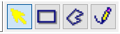 Select Mouse Mode
Use this set of mutual exclusive radio buttons to switch between four modes of mouse tool operation. Due to the fact that the two map display area are synchronized, any mouse actions performed on any of the map plot areas are automatically replicated on the other one.
- FOV/Pixel Selection Mode: Use this mouse mode to concomitantly zoom in and out the field of view (FOV) of the data and parameter maps, or to select the pixel coordinates for which the data spectrum and the GSFIT solution are displayed in the Spectral Fit panel.
- To zoom in, press, hold, move, and release the left mouse button to select the desired rectangular FOV (rubber-band selection process). To revert to the full FOV, use a single left-button click on any of the two map plots.
- Use a mouse right-click on any of the two map plots to make a pixel selection. The currently selected pixel is indicated by a set of horizontal and vertical dotted lines on both panels. Alternatively, the pixel may be selected using the Cursor X and Cursor Y numerical controls located below the data map plot area.
- Rectangular ROI Selection Mode: Use this mouse mode to define a rectangular region of interest (ROI) through a left button rubber-band selection process. The selected ROI is preserved and displayed as long it is not replaced by another ROI selection, or deleted by a single left button click.
- Polygonal ROI Selection Mode: Use this mouse mode to define the vertices of polygonal ROI through a series of sequential left button clicks. To finalize the process, use a right button click to define the last vertex, which will be automatically connected with the first one. The selected ROI is preserved and displayed as long it is not replaced by another ROI selection, or deleted by a single left button click.
- Free-hand ROI Selection Mode: Use this mouse mode to define an arbitrarily shaped ROI contour through a continues movement of the mouse cursor while the left button is pressed. To finalize the process, release the left button to define the last vertex of the countour, which will be automatically connected with the first one. The selected ROI is preserved and displayed as long it is not replaced by another ROI selection, or deleted by a single left button click.