EOVSA Data Analysis Tutorial
Browsing EOVSA data

Currently the most convenient way for browsing EOVSA data is through the RHESSI Browser. First, check the "EOVSA Radio Data" box on the data selection area (top-left corner). Then select year/month/date to view the overall EOVSA dynamic spectrum. Note if a time is selected at early UTC hours (e.g., 0-3 UT), it will show the EOVSA dynamic spectrum from the previous day. Also note that EOVSA data were not commissioned for spectroscopic imaging prior to April 2017. An example of the overview EOVSA dynamic spectrum for 2017 Aug 21 is shown in the figure on the right.
The overview EOVSA dynamic spectra shown are from uncalibrated cross-power visibilities at a few short baselines, which is a good proxy of, but not the total-power dynamic spectra. The effect of spatial information blended in the cross-power visibilities can be clearly seen as the "U"-shaped features throughout the day, which is due to the movement of the Sun across the sky that effectively changes the length and orientation of the baselines.
Flare times can be easily seen in the EOVSA dynamic spectra, which usually appear as vertical bright features across many frequency bands.
Software
We have developed two packages for EOVSA data processing and analysis:
- SunCASA A wrapper around CASA for imaging and visualizing spectral imaging data of the Sun. More information about CASA can be found on NRAO's CASA website . Note, (Sun)CASA is ONLY AVAILABLE on UNIX-BASED PLATFORMS (sorry Windows users).
- GSFIT A IDL-widget(GUI)-based spectral fitting package called gsfit, which provides a user-friendly display of EOVSA image cubes and an interface to fast fitting codes (via platform-dependent shared-object libraries).
There are two approaches in accessing our software packages. One is through our Amazon AWS server (recommended for participants of the EOVSA tutorial at the RHESSI 18 Workshop). Another is to install them on your own machine. We discuss the first approach in Section 1.1, and the second in Section 1.2.1 (SunCASA) and 1.2.2 (GSFIT).
Using Software on AWS server
We use an Amazon AWS Lightsail server for testing purposes. The server has 2 CPUs, 8 GB RAM, and 160 GB SSD storage. It runs CentOS 7 (1901-01) Linux. Please limit your usage to LIGHTWEIGHT DATA PROCESSING ONLY.
NOTE: THE ACCOUNT IS ONLY INTENDED FOR THE EOVSA TUTORIAL, BUT *NOT* FOR CARRYING OUT ACTUAL DATA REDUCTION
- Obtain SSH Key from Bin Chen
- Put it under a secure location on your own machine.
- Follow remaining directions depending on your client machine.
Connecting via Linux / Mac
Recommend to use "~/.ssh" (create if it does not exist by "mkdir ~/.ssh").
- Edit the permission of ~/.ssh and the key (here I use ~/.ssh as the directory to place your key)
chmod 700 ~/.ssh
chmod 400 ~/.ssh/guest-virgo.pem
- Log on to test AWS server (password-less)
ssh -X -i ~/.ssh/guest-virgo.pem guest@virgo.arcs.az.njit.edu
Now you are connected to virgo.
Connecting via Windows (MobaXterm)
Recommend to use "Documents\MobaXterm\home\.ssh", which should exist if you have already installed the free MobaXterm[1].
- Create new session, click SSH, enter virgo.arcs.az.njit.edu for Remote host, guest for username.
- On advanced SSH settings tab, click Use private key, navigate to and select file guest_key.pem
- Close setup window and click the new sessions icon, which will log you in.
Startup SunCASA and sswIDL
Once the connection is setup, you will have access to SunCASA and GSFIT (included in the sswIDL installation). To not interfere with others (who share the same "guest" account), please create your own directory and work under it. For easier identification, please use the initial of your first name and your full last name as the name (such as "bchen")
[guest@ip-172-26-5-203 ~]$ mkdir bchen
[guest@ip-172-26-5-203 ~]$ cd bchen
Enter SunCASA
[guest@ip-172-26-5-203 ~/bchen]$ suncasa
Enter sswIDL
[guest@ip-172-26-5-203 ~/bchen]$ sswidl
SunCASA Installation
Please click on the link above for details regarding installation of SunCASA on your own machine (only available on Unix-bases OS). This will take you to another page.
GSFIT Installation
Please click on the link above for details regarding installation of GSFIT on your own machine. This will take you to another page.
Spectral Imaging with SunCASA
Before Starting SunCASA
You will likely be running SunCASA from a working directory that has your data on it, or where you want your output to go. Warning: SunCASA does not like a directory that contains spaces in its path. If you have done your own installation as instructed above, then there should be an executable script called suncasa in your system path. This script will set up the required environment and run the version of SunCASA that it points to. EOVSA data is handled in CASA tables system, known as a Measurement Set (MS). The actual visibility data are stored in a MAIN table that contains a number of rows, each of which is effectively a single timestamp for a single spectral window and a single baseline. Within SunCASA, you will have access to a collection of tools that allow you to explore and utilize the new radio dynamic spectroscopic imaging data from EOVSA. You can open up a terminal, cd your working directory (e.g., ~/bchen/), and type
# in a terminal, outside of SunCASA:
cd yourworkdirectory
suncasa
Within SunCASA, you are using IPython to interact with the system. This does not mean extensive python experience is necessary. Basic Python interactions are straightforward, e.g., assigning parameters, importing modules, running functions.
Dynamic Spectrum and Imaging
Overview
This tutorial describes the making dynamic spectrum and imaging the EOVSA microwave data observed on August 21, 2017. The calibrated data set for the tutorial can be access on virgo. Please copy it over to you working directory.
## in SunCASA
!cp -r /common/data/eovsa_tutorial/IDB20170821201020-203020.12s.slfcaled.ms ./
Get Dynamic Sepctrum with SunCASA
The first module we introduce is dspec. This module allows you to generate a dynamic spectrum from an MS file, and visualize it. You can select a subset of data by specifying a time range, spectral windows/channels, antenna baseline, or uvrange. The selection syntax follows the CASA convention. More information of CASA selection syntax may be found in the above links or the Measurement Selection Syntax.

from suncasa.utils import dspec as ds
import matplotlib.pyplot as plt
## define the visbility data file
msfile = 'IDB20170821201020-203020.12s.slfcaled.ms'
## define the output filename of the dynamic spectrum
specfile = msfile + '.dspec.npz'
##  antenna selection
## leave it blank for selecting all baselines
bl = ''
## Spectral Windows and Channels selection
## leave it blank for selecting all spectral windows
spw = ''
## time range selection
## leave it blank for selecting the entire time interval
timeran = ''
## select baselines with a median length (0.15~0.5km)
uvrange = '0.15~0.5km'
## this step generates a dynamic spectrum and saves it to specfile
ds.get_dspec(vis=msfile, specfile=specfile, bl=bl, spw=spw, uvrange=uvrange)
## this plot the dynamic spectrum.
ds.plt_dspec(specfile, pol='XXYY')
## show the plot
plt.show()
Now you should have a popup window showing the dynamic spectrum. Hover your mouse over the dynamic spectrum, you can read the time and frequency information at the bottom of the window.
Imaging with SunCASA
Imaging EOVSA data involves image cleaning, as well as solar coordinate transformation and image registration. We bundle a number of imaging steps ino a module qlookplot. Now let us start with making a radio image from the spectral window 5 (5.4 GHz).
## in SunCASA
from suncasa.utils import qlookplot as ql
msfile = 'IDB20170821201020-203020.12s.slfcaled.ms'
vis = msfile
specfile = msfile + '.dspec.npz'  ## provide the dynamic spectrum data or it will generate a new one.
timerange = '20:21:10~20:21:30'  ## set the time interval
spw = '7'  ## select the spectral window 7
stokes = 'XXYY'   ## polarizations selection
ql.qlookplot(vis, specfile=specfile, timerange=timerange, spw=spw, stokes=stokes)
Spectral Fitting with GSFIT
GSFIT GUI Application
The GSFIT GUI application may be launched as follows
IDL> gsfit [,nthreads]
where nthreads is an optional argument that indicates the number of parallel asynchronous threads to be used when performing the fit tasks. By default, GSFIT launches with only one thread, but the user may interactively add or delete threads as needed at the run-time up to the number of CPUs available on the system (Note, if you are working on the AWS server, please use only one thread). After some delay while the interface loads, the GUI below should appear.
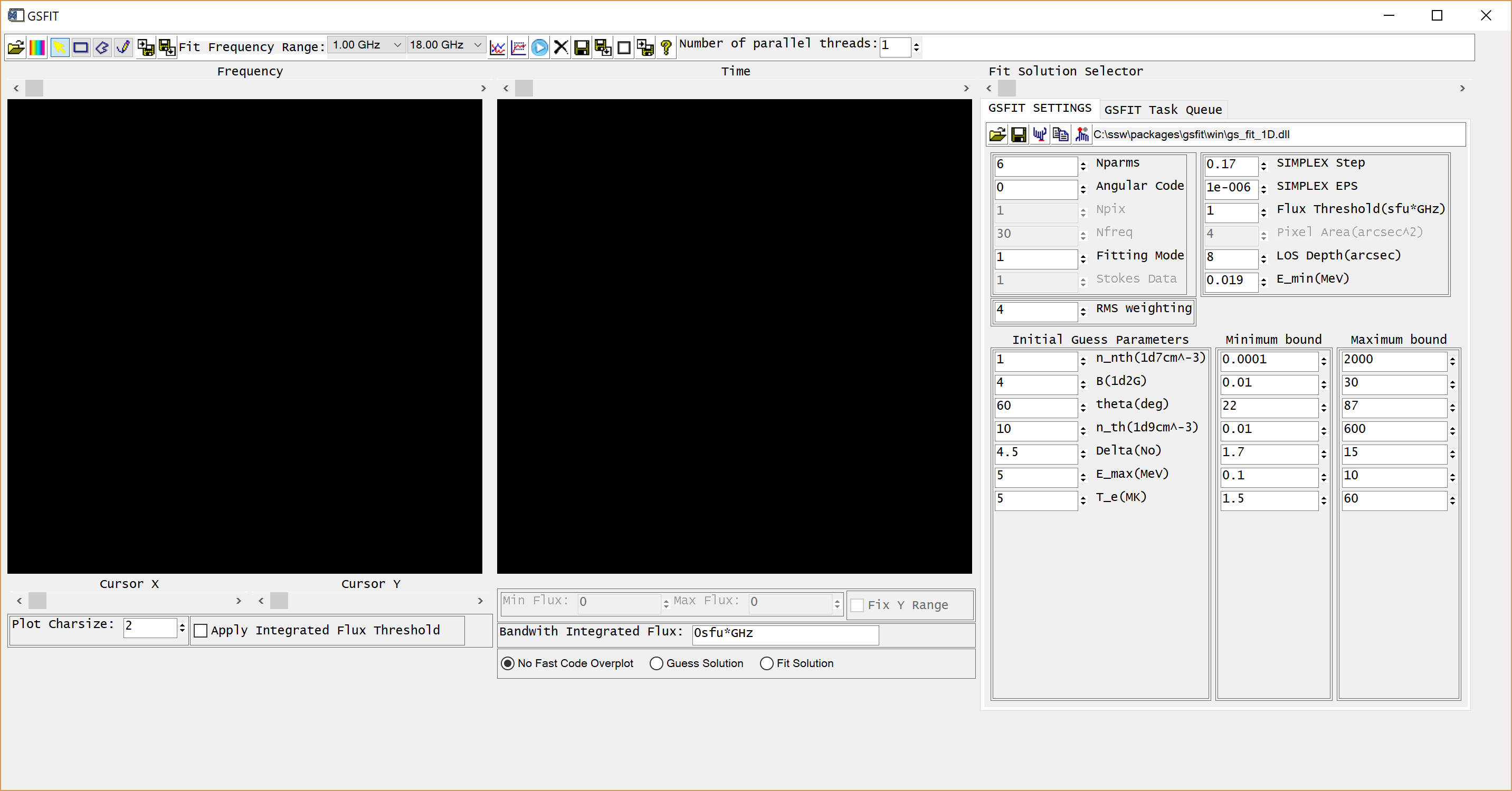
GSFIT GUI appearance on Windows OS
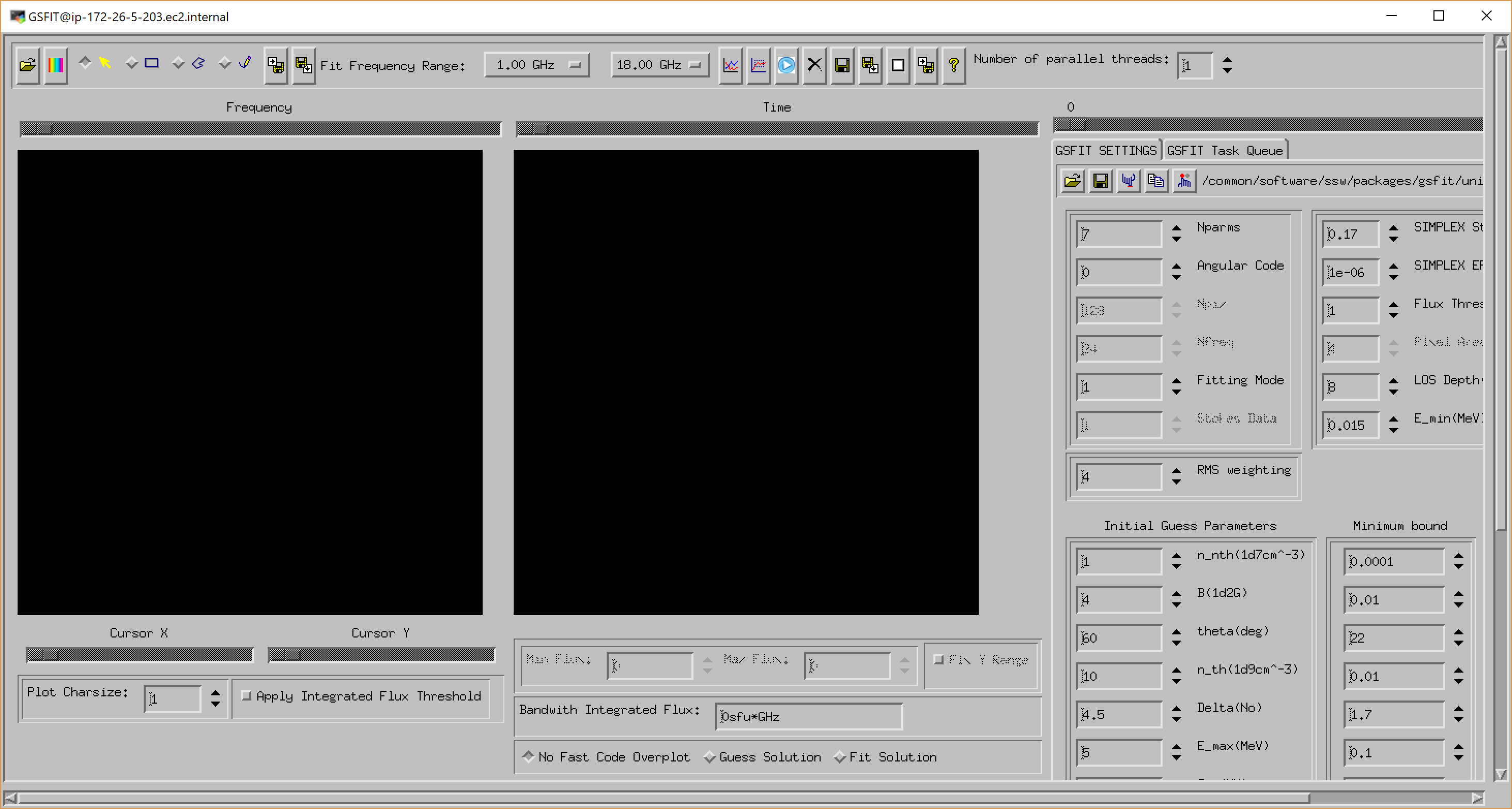
GSFIT GUI appearance on Linux/Mac OS


A detailed description of the GSFIT functionality is provided in the page linked below.
GSFIT Help
GSFITCP Batch Mode Application
GSFITCP is the command prompt counterpart of the GSFIT GUI microwave spectral fitting application. Once started, GSFITCP is designed to run in unattended mode until all fitting tasks assigned to it are completed and log on the disk in an user-defined *.log file, the content of which may be visualized using the GSFITVIEW GUI application. When run remotely on an Linux/Mac platform, the GSFITCP may be launched on a detached screen, which allows the remote user to logout without stopping the process in which GSFITCP runs.
GSFITCP is launched using the following call:
IDL> gsfitcp, taskfile, nthreads, /start
where taskfile is a path to a file in which a GSFIT task has been previously saved, as explained in the GSFIT Help page, nthreads is an optional argument indicating the number of parallel asynchronous threads to be used, and the optional keyword /start, if set, requests immediate start of the batch processing.
A detailed description of the GSFITCP functionality is provided in the page linked below.
GSFITCP Help
GSFITVIEW GUI Application
The GSFITVIEW GUI application may be launched as follows
IDL> gsfitview [,gsfitmaps]
where the optional gsfitmaps argument is either the filename of an IDL *.sav file containg a GSFIT Parameter Map Cube structure produced by the GSFIT or GSFITCP applications, or an already restored such structure.


A detailed description of the GSFITVIEW functionality is provided in the page linked below.