EOVSA Data Analysis Tutorial: Difference between revisions
| Line 12: | Line 12: | ||
=Calibrating EOVSA data= | =Calibrating EOVSA data= | ||
*<b>Calibration</b>: | *<b>Calibration</b>: Calibrating EOVSA data is an involved process. We are currently working on a semi-automatic pipeline for calibrating the visibility data. At this moment, however, please contact the EOVSA team if you wish to have calibrated visibility data for a specific event. In the near future, we envision the pipeline-calibrated visibility data to be available for download on a regular basis. | ||
*<b>Self-calibration</b>: For improving the quality of the imaging, self-calibration is usually needed. This is still a work-in-progress, but we have had some successful practice in self-calibrating some flare events. Please refer to [[Self-Calibrating Flare Data]] for examples and detailed discussions on our current practice for self-calibrating EOVSA flare data. | *<b>Self-calibration</b>: For improving the quality of the imaging, self-calibration is usually needed. This is still a work-in-progress, but we have had some successful practice in self-calibrating some flare events. Please refer to [[Self-Calibrating Flare Data]] for examples and detailed discussions on our current practice for self-calibrating EOVSA flare data. | ||
Revision as of 15:16, 24 May 2019
Browsing and Obtaining EOVSA data

Currently the most convenient way for browsing EOVSA data is through the RHESSI Browser. First, check the "EOVSA Radio Data" box on the data selection area (top-left corner). Then select year/month/date to view the overall EOVSA dynamic spectrum. Note if a time is selected at early UTC hours (e.g., 0-3 UT), it will show the EOVSA dynamic spectrum from the previous day. Also note that EOVSA data were not commissioned for spectroscopic imaging prior to April 2017. An example of the overview EOVSA dynamic spectrum for 2017 Aug 21 is shown in the figure on the right.
The overview EOVSA dynamic spectra are from the median of the uncalibrated cross-power visibilities at a few short baselines, which are not (but a good proxy of) the total-power dynamic spectra. The effects of spatial information blended in the cross-power visibilities can be clearly seen as the "U"-shaped features throughout the day, which are due to the movement of the Sun across the sky that effectively changes the length and orientation of the baselines. Flare times can be easily seen in the EOVSA dynamic spectra, which usually appear as vertical bright features across many frequency bands. More information can be found on this page.
We are currently working on a pipeline to create quicklook full-disk images for implementation at the RHESSI Browser in a way similar as the RHESSI quicklook images. Please stay tuned.
Once you identify the flare time, you can find the full-resolution (1-s cadence) uncalibrated visibility files (in Miriad format) at this link. Each data file is usually 10 minutes in duration. Name convention is YYYYMMDD/IDBYYYYMMDDHHMMSS, where the time in the file name indicates the start time of the visibility data.
Calibrating EOVSA data
- Calibration: Calibrating EOVSA data is an involved process. We are currently working on a semi-automatic pipeline for calibrating the visibility data. At this moment, however, please contact the EOVSA team if you wish to have calibrated visibility data for a specific event. In the near future, we envision the pipeline-calibrated visibility data to be available for download on a regular basis.
- Self-calibration: For improving the quality of the imaging, self-calibration is usually needed. This is still a work-in-progress, but we have had some successful practice in self-calibrating some flare events. Please refer to Self-Calibrating Flare Data for examples and detailed discussions on our current practice for self-calibrating EOVSA flare data.
Analyzing EOVSA data
Software
We have developed two packages for EOVSA data processing and analysis:
- SunCASA A wrapper around CASA (the Common Astronomy Software Applications package) for synthesis imaging and visualizing solar spectral imaging data. CASA is one of the leading software tool for "supporting the data post-processing needs of the next generation of radio astronomical telescopes such as ALMA and VLA", an international effort led by the National Radio Astronomy Observatory. The current version of CASA uses Python (2.7) interface. More information about CASA can be found on NRAO's CASA website . Note, CASA is available ONLY on UNIX-BASED PLATFORMS (and therefore, so is SunCASA).
- GSFIT A IDL-widget(GUI)-based spectral fitting package called gsfit, which provides a user-friendly display of EOVSA image cubes and an interface to fast fitting codes (via platform-dependent shared-object libraries).
For this tutorial, there are two approaches in accessing our software packages:
- 1. Through our Amazon Cloud server. See Section 3.1.1 for detailed instructions.
- 2. Install on your own machine. See Section 3.1.2 (SunCASA) and Section 3.1.3 (GSFIT) for instructions.
Using Software on Amazon Cloud Server
We use an Amazon AWS Lightsail cloud server for testing purposes. The server has 2 CPUs, 8 GB RAM, and 160 GB SSD storage. It runs CentOS 7 (1901-01) Linux. Please limit your usage to LIGHTWEIGHT DATA PROCESSING ONLY.
NOTE: the guest account is ONLY INTENDED FOR THE EOVSA TUTORIAL, WHICH WILL BE DISABLED SHORTLY AFTER THE RHESSI WORKSHOP (you will be notified prior to that). If you wish to continue using the server for testing purposes after the tutorial, please contact Bin Chen to set up a personal account.
DISCLAIMER: We are NOT RESPONSIBLE for any loss, damage, or leak of your personal data on the server.
- Obtain SSH Key to the guest account from Bin Chen
- Put it under a secure location on your own machine.
- Follow remaining directions depending on your client machine.
Connecting via command line
- Edit the permission of the SSH key and the directory you choose to place it. Here I use ~/.ssh as an example (create it first by mkdir ~/.ssh if it does not exist.)
chmod 700 ~/.ssh
chmod 400 ~/.ssh/guest-virgo.pem
- Log on to test AWS server (password-less)
ssh -X -i ~/.ssh/guest-virgo.pem guest@virgo.arcs.az.njit.edu
Now you are connected to virgo.
Connecting via Windows (MobaXterm)
Recommend to use "Documents\MobaXterm\home\.ssh", which should exist if you have already installed the free MobaXterm[1].
- Create new session, click SSH, enter virgo.arcs.az.njit.edu for Remote host, guest for username.
- On advanced SSH settings tab, click Use private key, navigate to and select file guest_virgo.pem
- Close setup window and click the new session's icon, which will log you in.
Startup SunCASA and sswIDL
Once you are connected to virgo, you will have access to SunCASA and GSFIT (included in the sswIDL installation). To not interfere with others (who share the same "guest" account), please create your own directory and work under it. For easier identification, please kindly use the initial of your first name and your full last name as the name of your directory (here "bchen" is used as an example).
[guest@ip-172-26-5-203 ~]$ mkdir bchen
[guest@ip-172-26-5-203 ~]$ cd bchen
To enter SunCASA
[guest@ip-172-26-5-203 ~/bchen]$ suncasa
To enter sswIDL
[guest@ip-172-26-5-203 ~/bchen]$ sswidl
SunCASA Installation
Please follow this link for details regarding installation of SunCASA on your own machine (only available on Unix-bases OS). This will take you to another page.
GSFIT Installation
Please follow this link for details regarding installation of GSFIT on your own machine (which supports multiple platforms). This will take you to another page.
Example Data and Scripts
In this tutorial, we will demonstrate steps for spectral imaging (self-)calibrated visibility data for a C-class flare on 2017 Aug 21 at ~20:20 UT (Section 3.3), followed by a tutorial on visualizing and analyzing the resulting spectral imaging cube (Section 3.4).
The visibility data can be accessed by
- Downloading from this Google Drive link.
- If you are on our AWS cloud server "virgo" (means for accessing the server are discussed in Section 3.1.1), it is located at /common/data/eovsa_tutorial/IDB20170821201800-202300.4s.slfcaled.ms.
To reduce the amount of data for this tutorial, the time resolution has been reduced by a factor of 4, to 4 s per sample. The actual time resolution available is 1 s. If you are on virgo, please copy it over to your own working directory that you created earlier under the guest account (e.g., ~/bchen/).
cd ''your_working_directory''
cp -r /common/data/eovsa_tutorial/IDB20170821201800-202300.4s.slfcaled.ms ./
Example scripts for doing the analysis covered in this tutorial are available as this Github repository. On Virgo, the scripts can be found under /common/data/eovsa_tutorial/.
Spectral Imaging with SunCASA
EOVSA data is handled in CASA tables system, known as a Measurement Set (MS). The actual visibility data are stored in a MAIN table that contains a number of rows, each of which is effectively a single timestamp for a single spectral window and a single baseline. Within SunCASA, in addition to everything already available in CASA, you have access to additional tools that allow you to explore and utilize the new radio dynamic spectroscopic imaging data from EOVSA. We also had success in using SunCASA for analyzing data from the Karl G. Jansky Very Large Array. The steps are very similar to those described here. To start SunCASA, use:
suncasa
Within SunCASA, you are under the IPython environment. Everything you know about (I)Python should be applicable here. The installation comes with frequently used packages including Matplotlib, Numpy, SciPy, AstroPy, SunPy. However, it is not very intuitive to add (compatible) Python packages within (Sun)CASA. If you choose to do so, you may want to check this page on how to install AstroPy (which is not originally shipped with CASA) within CASA. This method is generally applicable to adding other packages (but not thoroughly tested). If you need some specific packages for your analysis, and it does not require direct interaction with (Sun)CASA, we recommend you to use the standard Python environment. On Virgo, we have installed Anaconda 3, which can be accessed by, e.g., typing "ipython" in a terminal window.
Cross-Power Dynamic Spectrum
The first module we introduce is dspec. This module allows you to generate a cross-power dynamic spectrum from an MS file, and visualize it. You can select a subset of data by specifying a time range, spectral windows/channels, antenna baseline, or uvrange. The selection syntax follows the CASA convention. More information of CASA selection syntax may be found in the above links or the Measurement Selection Syntax.

from suncasa.utils import dspec as ds
import matplotlib.pyplot as plt
## define the visbility data file
msfile = 'IDB20170821201800-202300.4s.slfcaled.ms'
## define the output filename of the dynamic spectrum
specfile = msfile + '.dspec.npz'
## select relatively short baselines within a length (here I use 0.15~0.5km),
## and take a median cross all of them (with the domedian parameter)
## alternatively, you can use the "bl" parameter to select individual baseline(s)
uvrange = '0.15~0.5km'
## this step generates a dynamic spectrum and saves it to specfile
ds.get_dspec(vis=msfile, specfile=specfile, uvrange=uvrange, domedian=True)
## Other optional parameters are available for more selection criteria
## such as frequency range ("spw"), and time range ("timeran")
## Use "ds.get_dspec?" to see more options

## define the polarizations to show (here I use XX and YY)
pol='XXYY'
## The following command displays the resulting cross-power dynamic spectrum
ds.plt_dspec(specfile, pol=pol)
plt.show()
Now you should have a popup window showing the dynamic spectrum. Hover your mouse over the dynamic spectrum, you can read the time and frequency information at the bottom of the window.
Quick-Look Imaging
Imaging EOVSA data involves image cleaning, as well as solar coordinate transformation and image registration. We bundled a number of these steps ino a module named qlookplot, allowing users to generate an observing summary plot showing the cross power dynamic spectrum, GOES light curves and EOVSA quick-look images. Now let us start with making a summary plot of EOVSA image at the spectral window 5 (5.4 GHz).

## in SunCASA
from suncasa.utils import qlookplot as ql
msfile = 'IDB20170821201800-202300.4s.slfcaled.ms'
## (Optional) provide the save file for the cross-power dynamic spectrum.
## If not provided, the program will generate a new one from the visibility.
specfile = msfile + '.dspec.npz'
## set the time interval
timerange = '20:21:10~20:21:18'
## select frequency range from 5 GHz to 6 GHz
spw = '5~6GHz'
## select stokes XX
stokes = 'XX'
## turn off AIA image plotting, default is True
plotaia = False

ql.qlookplot(vis=msfile, specfile=specfile, timerange=timerange, spw=spw, \
    stokes=stokes, plotaia=plotaia)
Feel free to explore by adjusting the above parameters, e.g. use a different time range ("timerange" parameter) and/or frequency range ("spw" parameter).
With qlookplot, it is easy to engage solar data from SDO/AIA in the summary plot. Setting plotaia=True in the qlookplot command will download SDO/AIA data at the given time to current directory and add it to the summary plot.

## in SunCASA
ql.qlookplot(vis=msfile, specfile=specfile, timerange=timerange, spw=spw, \
    stokes=stokes, plotaia=True)
The resulting radio image is a 4-D datacube (in solar X-pos, Y-pos, frequency, and polarization), which is, by default, saved as a fits file msfile + '.outim.image.fits' under your working directory. The name of the output fits file can be specified using the "outfits" parameter. In this example, we combine all selected frequencies (specified in keyword "spw") into one image (i.e., multi-frequency synthesis). Therefore the third axis only has one plane. The fourth axis contains polarization. In this example, however, only the first one is populated ("XX"). Here is the relevant information in the header of the resulting FITS file.
NAXIS   =                    4
NAXIS1  =                  512/ Nx
NAXIS2  =                  512/ Ny
NAXIS3  =                    1/  number of frequency
NAXIS4  =                    2/  number of polarization
By default, qlookplot produces a full sun radio image (512x512 with a pixel size of 5"). If you know where the radio source is (e.g., from the previous full-Sun imaging), you can make a partial solar image around the source by specifying the image center ("xycen"), pixel scale ("cell"), and image field of view ("fov"). Here we show an example that images a 8-s interval around 20:21:14 UT using multi-frequency synthesis in 12-14 GHz and a smaller restoring beam. The microwave source is show to bifurcate into two components, which correspond pretty well with the double flare ribbons in SDO/AIA.

## in SunCASA
xycen = [375, 45]  ## image center for clean in solar X-Y in arcsec
cell=['2.0arcsec'] ## pixel scale
imsize=[128]   ## number of pixels in X and Y. If only one value is provided, NX = NY
fov = [100,100]  ## field of view of the zoomed-in panels in unit of arcsec
ql.qlookplot(vis=msfile, specfile=specfile, timerange='20:21:10~20:21:18', \
              spw='12GHz~14GHz', stokes='XX', restoringbeam=['6arcsec'],\
              imsize=imsize,cell=cell,xycen=xycen,fov=fov,calpha=1.0)
Next, we will make images for every single spectral window in this data set (from spw 1 to 30, spw 0 is in the visibility data, but is not calibrated for this event).

## in SunCASA
xycen = [375, 45]  ## image center for clean in solar X-Y in arcsec
cell=['2.0arcsec'] ## pixel size
imsize=[128]   ## x and y image size in pixels.
fov = [100,100]  ## field of view of the zoomed-in panels in unit of arcsec
spw = ['{}'.format(s) for s in range(1,31)]
clevels = [0.5, 1.0]  ## the contour levels of the transparent contours of the radio maps.
calpha=0.35  ## now tune down the alpha
ql.qlookplot(vis=msfile, specfile=specfile, timerange=timerange, spw=spw, stokes=stokes, \
            restoringbeam=restoringbeam,imsize=imsize,cell=cell, \
            xycen=xycen,fov=fov,clevels=clevels,calpha=calpha)
The output FITS file as a 4-d cube is saved to msfile + '.outim.image.fits' under your working directory. The 30 spectral windows used for spectral imaging are combined in the output FITS file. So NAXIS3 (frequency axis) is 30.
NAXIS   =                    4 / number of array dimensions
NAXIS1  =                  128
NAXIS2  =                  128
NAXIS3  =                   30
NAXIS4  =                    2
Batch-Mode Imaging
This section is for interested users who wish to generate FITS files with full control on all parameters being used for synthesis imaging. We provide one example SunCASA script for generating 30-band spectral imaging maps, and another for iterating over time to produce a time series of these maps.
Producing a 30-band map cube for a given time
An example script can be found at this Github link. If you are on the AWS server Virgo, it is under /common/data/eovsa_tutorial/imaging_example.py. First, download or copy the script to your own working directory and cd to your directory.
# in SunCASA
CASA <##>: cd your_working_directory
CASA <##>: !cp /common/data/eovsa_tutorial/imaging_example.py ./

Second (optional), change inputs in the following block in your copy of the "imaging_example.py" script and save the changes. This block has definitions for time range, image center and FOV, antennas used, cell size, number of pixels, etc.
################### USER INPUT GOES IN THIS BLOK ################
vis = 'IDB20170821201800-202300.4s.slfcaled.ms'  # input visibility data
trange = '2017/08/21/20:21:00~2017/08/21/20:21:30' # time range for imaging
xycen = [380., 50.] # center of the output map (in solar X and Y, Unit: arcsec)
xran = [280., 480.] # plot range in solar X. Unit: arcsec
yran = [-50., 150.] # plot range in solar Y. Unit: arcsec
antennas = '' # Use all 13 EOVSA 2-m antennas by default
npix = 256 # number of pixels in the image
cell = '1arcsec' # pixel scale in arcsec
pol = 'XX' # polarization to image, use XX for now
pbcor = True # correct for primary beam response?
outdir = './images' # Specify where to save the output fits files
outimgpre = 'EO' # Something to add to the output image name
Then, run the script in SunCASA via
CASA <##>: execfile('imaging_example.py')
The output fits images are saved under outdir. The naming conversion is outimgpre + YYYYMMDDTHHMMSS.SSS_S##.fits, where ## is the frequency band index number. See below for an example:
CASA <##>: ls ./images
EO20170821T202115.000_S01.fits  EO20170821T202115.000_S07.fits  EO20170821T202115.000_S13.fits  EO20170821T202115.000_S19.fits  EO20170821T202115.000_S25.fits
EO20170821T202115.000_S02.fits  EO20170821T202115.000_S08.fits  EO20170821T202115.000_S14.fits  EO20170821T202115.000_S20.fits  EO20170821T202115.000_S26.fits
EO20170821T202115.000_S03.fits  EO20170821T202115.000_S09.fits  EO20170821T202115.000_S15.fits  EO20170821T202115.000_S21.fits  EO20170821T202115.000_S27.fits
EO20170821T202115.000_S04.fits  EO20170821T202115.000_S10.fits  EO20170821T202115.000_S16.fits  EO20170821T202115.000_S22.fits  EO20170821T202115.000_S28.fits
EO20170821T202115.000_S05.fits  EO20170821T202115.000_S11.fits  EO20170821T202115.000_S17.fits  EO20170821T202115.000_S23.fits  EO20170821T202115.000_S29.fits
EO20170821T202115.000_S06.fits  EO20170821T202115.000_S12.fits  EO20170821T202115.000_S18.fits  EO20170821T202115.000_S24.fits  EO20170821T202115.000_S30.fits
From this point, you can use your favorite language (SSWIDL users: fits2map.pro would work on these) to read the fits files and plot them. The last block of the example script uses SunPy.map to generate the plot shown on the right.
Producing a time series of 30-band maps (a 4-d cube)
An example script can be found at this Github link. If you are on the AWS server Virgo, it is under /common/data/eovsa_tutorial/imaging_timeseries_example.py. The script enables parallel-processing (based on a customized task "ptclean3" -- do not ask me why we have "3" in the task name). To invoke more CPU processes for parallel-processing, change "nthreads" in the preambles from 1 to the number of threads you wish to use.
Caution: This script is very computationally intensive. Please do not try to run this script on the AWS server during the RHESSI 18 live tutorial, as it has limited resources that everyone must share.
# in SunCASA
CASA <##>: cd your_working_directory
CASA <##>: !cp /common/data/eovsa_tutorial/imaging_timeseries_example.py ./
Similar as the previous script, change inputs in the following block of your copy of the "imaging_timeseries_example.py" script and save the changes.

################### USER INPUT GOES IN THIS BLOK ####################
vis = 'IDB20170821201800-202300.4s.slfcaled.ms'  # input visibility data
specfile = vis + '.dspec.npz'  ## input dynamic spectrum
nthreads = 1  # Number of processing threads to use
overwrite = True  # whether to overwrite the existed fits files.
trange = ''  # time range for imaging, default to all times in the data
twidth = 1  # make one image out of every 2 time integrations
xycen = [380., 50.]  # center of the output map in solar X and Y. Unit: arcsec
xran = [340., 420.]  # plot range in solar X. Unit: arcsec
yran = [10., 90.]  # plot range in solar Y. Unit: arcsec
antennas = ''  # default is to use all 13 EOVSA 2-m antennas.
npix = 128  # number of pixels in the image
cell = '2arcsec'  # pixel scale in arcsec
pol = 'XX'  # polarization to image, use XX for now
pbcor = True  # correct for primary beam response?
grid_spacing = 5. * u.deg  # grid spacing in degrees
outdir = './image_series/'  # Specify where to save the output fits files
imresfile = 'imres.npz'  # File to write summary of the imaging results
outimgpre = 'EO'  # Something to add to the image name
Then, run the script in SunCASA by
CASA <##>: execfile('imaging_timeseries_example.py')
The output fits images and a summary file imresfile are saved under "outdir" (in this example "./image_timeseries"). The naming convention of output fits images is the same as the previous section. The summary yields the time, frequency, and path to every image.
CASA <##>: imres = np.load(outdir + imresfile)['imres'].item()
CASA <##>: imres.keys()
['FreqGHz', 'ImageName', 'Succeeded', 'BeginTime', 'EndTime']
CASA <##>: ls image_series/*.fits | head -5
image_series/EO20170821T201800.500_ALLBD.fits
image_series/EO20170821T201804.500_ALLBD.fits
image_series/EO20170821T201808.500_ALLBD.fits
image_series/EO20170821T201812.500_ALLBD.fits
image_series/EO20170821T201816.500_ALLBD.fits
The last block of the example script uses SunPy.map to generate a series of plots and wraps them as a javascript movie.
Plotting Images in SSWIDL
All the output files are in standard FITS format in the Helioprojective Cartesian coordinate system (that most spacecraft solar image data adopt; FITS header CTYPE is HPLN-TAN and HPLT-TAN). They are fully compatible with the SSWIDL map suite which deals with FITS files. We have prepared SSWIDL routines to convert the single time or time-series FITS files to an array of SSWIDL map structure. The scripts are available in the Github repository of our tutorial. For those working on Virgo, local copies are placed under /common/data/eovsa_tutorial/. Two scripts are relevant to this tutorial:
- casa_readfits.pro: read an array of multi-frequency FITS files into FITS header (index) and data.
- casa_fits2map.pro: convert an array of multi-frequency FITS files into an array of SSWIDL map structure (adapted from P. T. Gallagher's hsi_fits2map.pro)
First, start SSWIDL from command line:
sswidl
Find and convert the fits files:
; cd to your path that contains casa_readfits.pro and casa_fits2map.pro. If on Virgo, just add the path
IDL> add_path, '/common/data/eovsa_tutorial/'
IDL> fitsdir = '/common/data/eovsa_tutorial/image_series/'
IDL> fitsfiles = file_search(fitsdir+'*_ALLBD.fits')
; The resulting fitfiles contains all multi-frequency FITS files under "fitsdir"
; The following command converts the fits files to an array of map structures.
; "casa_fits2map.pro" also work well on a single FITS file.
; (Optional) keyword "calcrms" is to calculate rms and dynamic range (SNR) of the maps in a user-defined "empty" region
;        of the map specified by "rmsxran" and "rmsyran"
IDL> casa_fits2map, fitsfiles, eomaps[, /calcrms, rmsxran=[260., 320.], rmsyran=[-70., 0.]]
; Save the output maps as an IDL save file for future use
IDL> save,file='EOMAPS_20170821T201800-202300.4s.sav',eomaps
The resulting maps have a shape of [# of frequencies, # of polarizations, # of times]
IDL> help,eomaps
EOMAPS          STRUCT    = -> <Anonymous> Array[30, 1, 75]
They have compatible keywords recognized by, e.g., plot_map.pro. Example of the output map keywords:
IDL> help,eomaps,/str
** Structure <3bcf8e8>, 29 tags, length=131384, data length=131380, refs=1:
   DATA            DOUBLE    Array[128, 128]
   XC              DOUBLE           378.99123
   YC              DOUBLE           49.005429
   DX              DOUBLE           2.0000000
   DY              DOUBLE           2.0000000
   TIME            STRING    '21-Aug-2017 20:18:00.500'
   ID              STRING    'EOVSA XX 3.413GHz'
   DUR             DOUBLE           4.0000003
   XUNITS          STRING    'arcsec'
   YUNITS          STRING    'arcsec'
   ROLL_ANGLE      DOUBLE           0.0000000
   ROLL_CENTER     DOUBLE    Array[2]
   FREQ            DOUBLE           3.4125694
   FREQUNIT        STRING    'GHz'
   STOKES          STRING    'XX'
   DATAUNIT        STRING    'K'
   DATATYPE        STRING    'Brightness Temperature'
   BMAJ            DOUBLE        0.0097377778
   BMIN            DOUBLE        0.0097377778
   BPA             DOUBLE           0.0000000
   RSUN            DOUBLE           948.03949
   L0              FLOAT           0.00000
   B0              DOUBLE           6.9298481
   COMMENT         STRING    'Converted by CASA_FITS2MAP.PRO'
   RMS             DOUBLE           22995.481
   SNR             DOUBLE           92.201139
   RMSUNIT         STRING    'K'
   RMSXRAN         FLOAT     Array[2]
   RMSYRAN         FLOAT     Array[2]

An example for plotting all images at a selected time:
; choose a time pixel
IDL> plttime = anytim('2017-08-21T20:21:15')
IDL> dt = min(abs(anytim(eomaps[0,0,*].time)-plttime),tidx)
; use maps at this time, first polarization, and all bands
IDL> eomap = reform(eomaps[*,0,tidx])
IDL> window,0,xs=1000,ys=800
IDL> !p.multi=[0,6,5]
IDL> loadct, 3
IDL> for i=0, 29 do plot_map,eomap[i],grid=5.,$
         tit=string(eomap[i].freq,format='(f5.2)')+' GHz', $
         chars=2.0,xran=[340.,420.],yran=[10.,90.]
Spectral Fitting with GSFIT
In this section we discuss using GSFIT (now a package of SSWIDL) to perform spectral fit based on the resulting FITS images produced from the previous steps. We will use the IDL save file produced in Section 3.3.3.3 as the input. A copy of the IDL save file can be downloaded from this link. On Virgo, the IDL save file is located at /common/data/eovsa_tutorial/EOMAPS_20170821T201800-202300.4s.sav.
GSFIT GUI Application
The GSFIT GUI application may be launched as follows
IDL> gsfit [,nthreads]
where nthreads is an optional argument that indicates the number of parallel asynchronous threads to be used when performing the fit tasks. By default, GSFIT launches with only one thread, but the user may interactively add or delete threads as needed at the run-time up to the number of CPUs available on the system (Note, if you are working on the AWS server, please use only one thread). After some delay while the interface loads, the GUI below should appear.
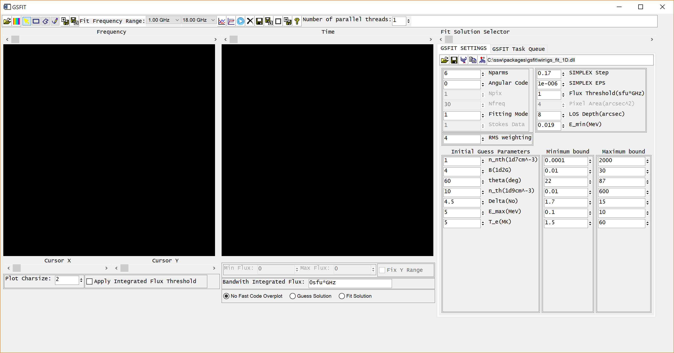
GSFIT GUI appearance on Windows OS
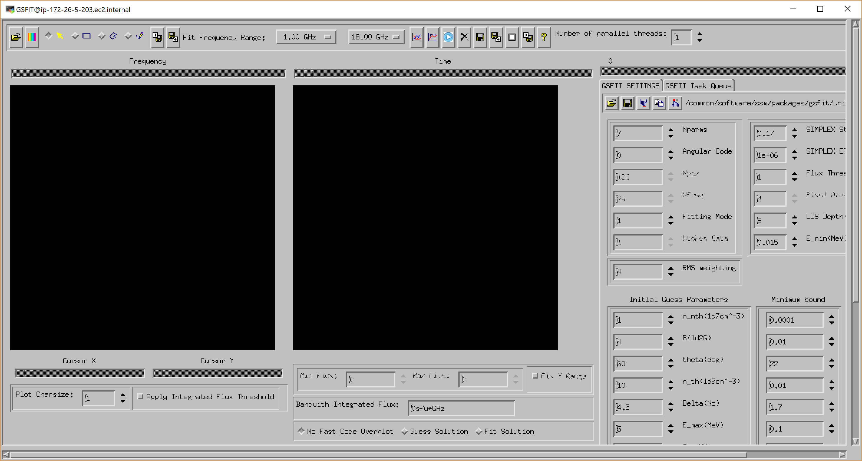
GSFIT GUI appearance on Linux/Mac OS


A detailed description of the GSFIT functionality is provided in the page linked below.
GSFIT Help
GSFITCP Batch Mode Application
GSFITCP is the command prompt counterpart of the GSFIT GUI microwave spectral fitting application. Once started, GSFITCP is designed to run in unattended mode until all fitting tasks assigned to it are completed and log on the disk in an user-defined *.log file, the content of which may be visualized using the GSFITVIEW GUI application. When run remotely on an Linux/Mac platform, the GSFITCP may be launched on a detached screen, which allows the remote user to logout without stopping the process in which GSFITCP runs.
GSFITCP is launched using the following call:
IDL> gsfitcp, taskfile, nthreads, /start
where taskfile is a path to a file in which a GSFIT task has been previously saved, as explained in the GSFIT Help page, nthreads is an optional argument indicating the number of parallel asynchronous threads to be used, and the optional keyword /start, if set, requests immediate start of the batch processing.
A detailed description of the GSFITCP functionality is provided in the page linked below.
GSFITCP Help
GSFITVIEW GUI Application
The GSFITVIEW GUI application may be launched as follows
IDL> gsfitview [,gsfitmaps]
where the optional gsfitmaps argument is either the filename of an IDL *.sav file containg a GSFIT Parameter Map Cube structure produced by the GSFIT or GSFITCP applications, or an already restored such structure.


A detailed description of the GSFITVIEW functionality is provided in the page linked below.