EOVSA Imaging Workshop
Software and sample data
Here are some basic information on CASA and the software we are developing:
- Obtaining CASA; CASA Guides
- suncasa A CASA/python-based package being developed for imaging and visualizing spectral imaging data. A useful (but potentially buggy) routine (helioimage2fits.py) is available for registering EOVSA/VLA (and ALMA) CASA images.
Software setup
For Unix platform users
For local people, you can ssh onto pipeline (@Owens Valley) or our local server baozi.hpcnet.campus.njit.edu and launch CASA. Everything has been set up already. The following instructions are for people who want to (or have to) set up their environment.
- Download the latest version of CASA. I'm using version 4.7.0, but the latest version should work.
CASA does not have EOVSA observatory information for this moment. You can manully add EOVSA observatory information in CASA,
# In CASA
import os
obsdict = {'MJD': 57447.0, 'Name': 'EOVSA', 'Type': 'WGS84', 'Long': -118.287, 'Lat': 37.2332, 'Height': 1207.13, 'X': 0.0, 'Y': 0.0, 'Z': 0.0, 'Source': 'Dale Gary'}
obstable = os.getenv("CASAPATH").split(' ')[0]+"/data/geodetic/Observatories"
tb.open(obstable,nomodify=False)
nrows = tb.nrows()
tb.addrows(1)
for k in obsdict.keys():
	tb.putcell(k,nrows,obsdict[k])
tb.close()
or download this, unzip (as Observatories), and place the directory under the folder where CASA stores its geodetic information. The folder can be found from a CASA prompt.
# In CASA
print os.getenv("CASAPATH").split(' ')[0]+"/data/geodetic/"
- Download the suncasa package from the GitHub page, and put it under <YOURPATH> as suncasa
- Incorporate suncasa into CASA:
Create ~/.casa/init.py -- this is a convenient way to put in any python codes you want to run whenever CASA is initialized (you can also do this manually after launching CASA)
# In CASA
import sys
sys.path.append('<YOURPATH that contains suncasa>')
- helioimage2fits calls astropy and sunpy within CASA. However, earlier versions of CASA (<5.0) does not have Astropy, and no version has sunpy. So we have to install Sunpy, and possibly also Astropy (depending on your CASA version)
- Install SunPy and/or Astropy into CASA. If you do not have Sunpy or Astropy in your python installation, the most convenient way to do so is through Anaconda (which would be your python version). If you don't have Anaconda, refer to this installation guide. With Anaconda in place, do the following to install Sunpy and Astropy
# In SHELL
conda config --add channels conda-forge
conda install sunpy
conda install astropy
Next, to call Sunpy and Astropy within CASA, we also need to add their paths to CASA's search path. This is done by adding your installed anaconda "site-packages" to ~/.casa/init.py. On a Mac, the default path is "~/anaconda/lib/python2.7/site-packages"
sys.path.append('/<FULL PATH TO YOUR CONDA python site-package>/site-packages')
Note: "~" for the home directory does not work for the line above. You need to make replace it with the full path or use the Python function os.path.expanduser() to find it.
Another way to install SunPy or AstroPy is as following -- unfortunately, this may fail if the CASA version does not match the most updated sunpy version.
# In CASA
from setuptools.command import easy_install
easy_install.main(['--user', 'pip'])
import pip
pip.main(['install', 'astropy'])
pip.main(['install', 'sunpy''])
- if nothing goes wrong, you've completed the installation! Now try and see if you can call suncasa.utils.helioimage2fits in CASA as follows
from suncasa.utils import helioimage2fits as hf
If there is no complain, you have successfully installed CASA, Sunpy, Astropy, and suncasa!
- In SUNCASA, we wrapped some useful python routines to customed CASA tasks, e.g., ptclean, pmaxfit. You can configure your CASA setup to automatically load these tasks on startup, so that they're always available to you.
# In SHELL
cd /<YOURPATH>/suncasa/tasks
buildmytasks
After buildmytasks has completed, there is now a configure file called "mytasks.py", which is the meta-file for all the tasks you might have in this directory. Add the following line to your ~/.casa/init.py file.
execfile('/<YOURPATH>/suncasa/tasks/mytasks.py')
For Windows platform users
Unfortunately, CASA works only on Unix platform. You can first install a virtual machine software to run a Unix operating system and follow the aforementioned guidance for Unix platform to install the CASA and suncasa.
- Download VirtualBox and install it on your windows machine.
- Install Ubuntu system to the VirtualBox. A quick tutorial can be found here. (Thanks to Jim and Gregory)
Data description and data access
To get started, we have made some calibrated flare and active region data in CASA measurement set format, available here. Here are some things to consider when working with the data:
- Antennas 1-8 and 12 have a wide sky coverage, while antennas 9-11 and 13 are the older equatorial mounts that can only cover +/- 55 degrees from the meridian. All antennas were tracking for the flare, but for portions of the all-day scan (roughly before 1600 UT or after 2400 UT) only 9 antennas will be tracking. Data for non-tracking antennas is NOT flagged, so if you try to image these periods, you'll need to manually omit ants 9-11 and 13.
- Because of the 2.5 GHz high-pass filters, data are taken only for bands 4-34. These will be labeled spectral window (spw) 0-31 in the measurement sets. However, band 4 (spw 0) is currently not calibrated, so only the 31 spectral windows 1-31 (bands 5-34, or frequencies 3-18 GHz) are valid data. You'll need to omit spw 0 when making images.
- In principle, circular polarization should be valid and meaningful, but no polarization calibration has been done (yet) so no non-ideal behavior (leakage terms, etc.) have been accounted for.
Flare Data
Folder Flare_20170910 contains four measurement sets at full 1-s time resolution, each with 10-min duration:
- IDB20170910154625.corrected.ms (171 MB) [1] containing the first 10 minutes of the flare (15:46:25-15:56:25 UT), calibrated but no self-calibration
- IDB20170910154625.corrected.ms.xx.selfcaled (66 MB) [2] self-calibrated data for polarization XX
- IDB20170910155625.corrected.ms (232 MB) [3] containing the second 10 minutes of the flare (15:56:25-16:06:25 UT)
- IDB20170910155625.corrected.ms.xx.selfcaled (77 MB) [4] self-calibrated data for polarization XX
All Day Quiet Sun/Active Region Data
Folder AR_20170710 contains 8 calibrated measurements sets at 60-s time resolution.
- The seven UDB20170710*.corrected.ms are files for each scan separately, ranging in size from 7 - 150 MB depending on the length of the scan.
- UDB20170710_allday.ms (268 MB) [5] is the same data concatenated into a single file. However, each scan has a separate source ID.
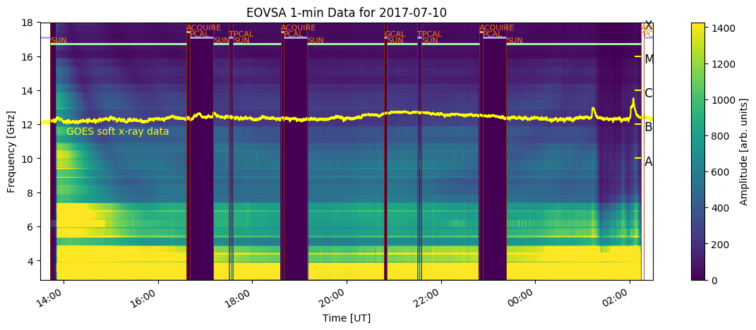
The AR data are also calibrated but not self-calibrated. In fact, we need to create a strategy for self-calibration of such data. You can get an overview of the AR coverage on that day by looking at the plot at http://ovsa.njit.edu/flaremon/daily/2017/XSP20170710.png. The separate scan files above are labeled with the time of the start of the scan, and each scan covers the time of continuous solar data between each calibration scan.
Make your first EOVSA flare image
Download this CASA script. It does basic clean on the full Sun using this slfcaled measurement set data near the flare peak (1600 UT) with 10-s integration, as well as image registration (into standard FITS file with helioprojective coordinates), and plotting using sunpy.

In CASA, cd to your data directory and do the following
execfile('imaging_example_20170910T1600.py')
You are supposed to see a plot similar to the one on the right. I have tested the script on both our servers on campus and Owens Valley. If not, something went wrong, most likely due to compatibility issues...
Possible Topics
We think that the best approach to the imaging workshop is not for everyone to work on the same topic, but rather to consider (and perhaps prioritize) different topics and then put together small teams of people who might be interested in investigating them. Here is a list of some possible topics, but in no prioritized order. Many topics will be somewhat interconnected, but we should avoid time-wasting situations where people working on one topic have to wait until another, uncompleted topic is done.
Calibration
Most calibrations needed for basic imaging are well in hand, so additional efforts are not really needed for an imaging workshop. Here is a list of (semi-)automatic calibrations we are doing so far. All can be improved, but such improvements will not make any major qualitative difference in the images.
- Gain corrections: To account for changes of the attenuation settings (esp. during flares). See this page for details.
- Correcting for polarization mixing due to feed rotation: See this page for details.
- Antenna-based amplitude calibration: made by referencing total power and auto-correlation amplitudes to RSTN/Penticton total solar flux density measurements. See this page for details.
- Reference phase calibration: antenna-based, band-averaged phases derived from "reference" observations of strong celestial radio sources every night. See this page for details]
- Daily phase calibration: antenna-based multi-band delays resulting from the phase difference as a function of frequency between those derived from phase calibrators (usually observed 3 times during the day) and the reference calibrator. See this page for details.
There are, however, two other calibrations still being developed:
- Polarization calibration: To calibrate absolute degree of circular polarization. We believe that the information already exists in available data, but the procedures need to be worked out. Additional observations are possible during this week, if needed.
- Per-channel bandpass (or single-band-delay) calibration within individual bands: To calibrate the phase/amplitude variations from one science channel to another. Procedures need to be worked out.
- Real-time spectral-kurtosis flagging of RFI, and other forms of RFI excision.
Pipeline Imaging
We have developed the basis for pipeline imaging of data on a daily basis, examples of the 2017 Jul 10 data can be seen here. These 10-min averages at a few bands might be okay, but lots of improvement is needed. Mainly, these improvements should be in the form of better imaging strategies (which are the subject of some of the topics below), and in better data-quality checks. In addition to these 10-min average images, we also envision making shorter (10-s?) images at a few bands during flares. Some of the RHESSI experience might come in handy here. Improving and finalizing the pipeline imaging is a high priority for this meeting!
Current sequence of creating daily 10-m cadence quicklook images
On pipeline, launch CASA
from suncasa.eovsa import eovsa_pipeline as ep
date='2017-07-10'
vis_corrected = ep.calib_pipeline(date, doimport=True)
ep.qlook_image_pipeline(date)
The resulting quicklook fits files are under /data1/eovsa/qlookfits/yyyy/mm/dd/, and the quicklook images are online at http://www.ovsa.njit.edu/qlookimg_10m/
Whole-day all-band frequency synthesis image (under development)
concateovsa(vis=[A list of ms files from one day],concatvis="UDBYYYYMMDD_allday.ms",datacolumn="corrected")
Flare Imaging
We have succeeded in making flare multi-frequency movies, which are extremely interesting and revealing, but are quite time-consuming and human-intensive. We need strategies to reduce the number of parameters for different imaging cases, and perhaps to automate or aid in clean-box choices. When converting data-cubes to spatially-resolved spectra, issues of total power calibration come into play.
Self-calibration Strategies
(Bin) Currently I am using a sliding window of five bands (band_to_selfcal +- 2 bands) to create a multi-frequency synthesized image as the input model for doing self-calibration at the band in question. Any alternative strategies? How about channel-by-channel selfcal?
Imaging Strategies
Clean? MEM? Optimum way to do spectral imaging? Here is an example made for the Sep 10 flare (Bin).
Quiet Sun and Active Region Imaging
We desperately need help in this area. We have made simple AR images that are quite promising, but full-disk images are still quite bad. Stephen can probably do wonders, and hopefully teach us to do so also. We should explore the use of additional data (say full-disk images from GAVRT) and how that might be used. How do we handle the issue of solar rotation, which can move an active region by multiple arcminutes over a 12-h day?
Self-calibration Strategies
We can probably do some self-calibration based on bright AR, but can we self-calibration on the solar disk? Gordon would like to explore the self-cal corrections vs. time, but it requires someone succeeding in doing an all-day self-calibration in the first place.
Imaging Strategies
Given solar rotation, and the limitations of EOVSA uv coverage, what are the best imaging strategies for full-disk and AR imaging?
Software Development
Currently we are using Python for analyzing calibration data and CASA for script-based imaging.
- What is the best approach to make an interactive imaging tool to serve the community (for both experts and non-experts)?
- How about the tool to visualize/analyze/make use of the resulted 4-D dynamic spectral imaging data?
Notes
Imaging Priority order
- flare selfcal Tim
- active region rotation Stephen
- solar disk model Stephen
- pipeline heuristics Group (Thurs. morning)
Three types of users to keep in mind
- want packaged data without further processing (catalog data)
choices made for user, such as standard set of bands, (png and fits images and fits dynamic spectrum of flares)
- parameters of their choosing, but without knowing intricacies of instrument (gui)
- Black-belt user who goes back to raw data, but not often doing their own calibration
- pipeline quicklook Bin, Sijie, Sa"m
Two levels of quicklook at standard frequencies
- Full-disk 10-min, limited resolution
- Zoomed-in 1-min, full resolution (requires locating in space and time)
- pipeline parallelization optimization
- visibility weighting
- user interface Jim, Sa"m
Action Item
Create FITS file of daily spectra. (Jim $$$)
Calibration Priority order
- polarization calibration Sam
- total power calibration
- relative vs spectrum Gordon
- gain calibration Gordon
- RFI excision Gelu, Gordon, Jim
Tim's Notes
Pipeline imaging
Most of the effort appeared to go into a standard selection of quiet Sun maps at 4-6 frequency ranges at a cadence of 10 min. Bin and I found that short baselines could have a large impact on the quality of the image due to their sparse sampling and large amplitudes. Going forward, I think the pipeline should routinely subtract models (see below) of (frequency-dependent) background disks from the data, map and clean the residual, and then add the model disk back. Removal of the background disk before mapping and cleaning would remove the problems associated with sparse sampling of short baselines.
Question 1: for those days when there are ARs present on the disk, should the pipeline produce quicklook maps of the individual ARs at higher resolution a la the Solar Monitor?
Question 2: is it worth investing some effort in correcting for solar rotation so that higher fidelity AR maps can be constructed using longer intervals of data?
For both pipeline AR imaging and the more general problem of QS imaging, some work needs to be done on optimizing weighting parameters; i.e., the "robust" parameter used in Briggs weighting and, possibly, a uv taper. We should also consider what type of clean beam to restore with. Currently, the pipeline restores a symmetrical beam that scales with frequency. It is conservative in the sense that the fitted beam is elliptical with an axial ratio of a:b~2:1. The symmetrical beam uses the larger dimension (a:a). It might be preferable to restore with the fitted beam or with a slightly higher resolution beam with a width sqrt(ab).
As we discussed, the quicklook data should be calibrated in units of brightness.
It is premature to get into the weeds on pipeline imaging of flares since they can span such a wide range of phenomenology. Nevertheless, it should be relatively straightforward to produce a suite of reference images or non-optimized movies at selected frequencies along with a dynamic spectrum that can be browsed to show the (polarized?) total power spectrum in another window.
Summary Notes on pipeline
We will do 4-band images each 10 min over each day, as quicklook images/movies. Both png and fits will be available, with links on data archive page. We should also have a Sun Today page.
Flare quicklook images will require a person to identify peak time, start and end time, and location (possibly done automatically from HEK). A single command with parameters should produce images/movie of the flare each 10 s.
We want calibrated total power spectrum, in fits format for each flare.
We want a single all-day, all-band full-disk image each day for imaging quality check.
Robust weighting
This came up because I noticed that, currently, all visibilities are assigned the same integer weights. For ALMA and the VLA, the weight is a statistical weight (variance) based on Tsys, bandwidth, integration time, etc. It is used in imaging to form a "robust" weighting of the visibilities to optimize the angular resolution and noise properties of the map. After playing around with it a bit I don't think it's worth pursuing in detail at this point. EOVSA is dominated by the source and so the weights should be the same for each visibility (how much does Tsys in fact vary because of Trx and pointing?). Moreover, imaging will usually be confusion limited, not limited by thermal noise. I can recommend a specific value for, e.g., the pipeline after I look at it a bit more.
Summary Notes
We will defer this to later.
Selfcal
It should be possible to selfcal most flares and so a standard set of heuristics should be established for doing so. Since flares vary in time and one is interested in the variation of the (spatially-resolved) spectrum with time, one is usually stuck with sparse sampling and the limitations that come with it. Based on his experience with the Sep 10 flare, Bin found that the model used for self-calibration benefited from frequency synthesis (FS): i.e., he formed a model image for frequency i by including frequencies i-2, i-1, i, i+1, and i+2, spanning 2 GHz. This improved the performance of selfcal and led to smoother spectra. A worry is that by using a model that includes data spanning a significant fractional bandwidth one might introduce significant bias into the self-calibrated data. For example, if the source location varies with frequency and the spectrum shows a significant slope across the 2 GHz used in the model, the source position of the self-calibrated data at frequency i could be affected.
I looked at this a bit using FS over 1, 3, 5, and 7 frequencies. More work needs to be done but my preliminary impression is that the lower frequencies were not strongly biased (for the Sep 10 example) but there may be problems at higher frequencies.
QS Model Fitting
I wrote an AIPS program long ago to fit a disk model to Nobeyama RH data. It fits for the center coordinate (X0, Y0), the radius, and the total flux although any of the parameters can be held fixed. The reason for fitting (X0,Y0) is that the NoRH uses redundant calibration and the images are therefore affected by the sky, resulting in jitter from integration to integration. For EOVSA, it should not be necessary to fit for (X0,Y0). In fact, with the total flux known at each frequency, it should only be necessary to fit for the radius as a function of frequency. This would, in fact, be a nice side project: mean solar radius as a function of frequency (and, longer term, phase in the solar cycle). EOVSA will be taking lots of QS data (unfortunately) and so it should be possible to use full scan data to produce very nice fits. These can be used as part of the standard pipeline (or user) data reduction to subtract out the background Sun, thereby simplifying imaging and deconvolution of AR or QS phenomena. The old code can maybe be used to demo all this but you'll probably want to write your own fitting routine. The data look very clean and fitting (and error estimation) should be straightforward.
I am interested in getting some QS data to play with. The Jul 10 data are nice but contain a large AR. Better to use truly quiet data. We looked at Jan 2 but ran into trouble with apparent calibration issues, the origin of which are not yet understood. It looks as though data from July 3-4 is quiet, so if Sijie or someone could get those to me, I would appreciate it.
Summary Notes
We identified some possible scaling issues based on total power calibration, that need to be checked. Disk fitting should wait for those checks to be completed.
Data Visualization
We didn't talk about this a lot. I assume that, for flares, science data will take the form of hypercubes (x, y, t, freq, pol'n) that can be manipulated, sliced, and diced using a tool suite that has yet to be developed. Some sort of interface to modeling software will also be needed. Don't know about active regions beyond the quicklook data...